Simplifying lists

library(tidyverse)
library(httr)
library(repurrrsive)

set.seed(123)
theme_set(theme_minimal())

Run the code below in your console to download this exercise as a set of R scripts.

usethis::use_course("cis-ds/getting-data-from-the-web-api-access")

Not all lists are easily coerced into data frames by simply calling content() %>% as_tibble(). Unless your list is perfectly structured, this will not work. Recall the OMDB example:

sharknado <- GET(
  url = "http://www.omdbapi.com/?",
  query = list(
    t = "Sharknado",
    y = 2013,
    apikey = getOption("omdb_key")
  )
)

# convert to data frame
content(sharknado, as = "parsed", type = "application/json") %>%
  as_tibble()

## # A tibble: 2 × 25
##   Title    Year  Rated Relea…¹ Runtime Genre Direc…² Writer Actors Plot  Langu…³
##   <chr>    <chr> <chr> <chr>   <chr>   <chr> <chr>   <chr>  <chr>  <chr> <chr>  
## 1 Sharkna… 2013  Not … 11 Jul… 86 min  Acti… Anthon… Thund… Ian Z… When… English
## 2 Sharkna… 2013  Not … 11 Jul… 86 min  Acti… Anthon… Thund… Ian Z… When… English
## # … with 14 more variables: Country <chr>, Awards <chr>, Poster <chr>,
## #   Ratings <list>, Metascore <chr>, imdbRating <chr>, imdbVotes <chr>,
## #   imdbID <chr>, Type <chr>, DVD <chr>, BoxOffice <chr>, Production <chr>,
## #   Website <chr>, Response <chr>, and abbreviated variable names ¹Released,
## #   ²Director, ³Language
## # ℹ Use `colnames()` to see all variable names

Wait a minute, what happened? Look at the structure of content():

content(sharknado) %>%
  str()

## List of 25
##  $ Title     : chr "Sharknado"
##  $ Year      : chr "2013"
##  $ Rated     : chr "Not Rated"
##  $ Released  : chr "11 Jul 2013"
##  $ Runtime   : chr "86 min"
##  $ Genre     : chr "Action, Adventure, Comedy"
##  $ Director  : chr "Anthony C. Ferrante"
##  $ Writer    : chr "Thunder Levin"
##  $ Actors    : chr "Ian Ziering, Tara Reid, John Heard"
##  $ Plot      : chr "When a freak hurricane swamps Los Angeles, nature's deadliest killer rules sea, land, and air as thousands of s"| __truncated__
##  $ Language  : chr "English"
##  $ Country   : chr "United States"
##  $ Awards    : chr "1 win & 2 nominations"
##  $ Poster    : chr "https://m.media-amazon.com/images/M/MV5BODcwZWFiNTEtNDgzMC00ZmE2LWExMzYtNzZhZDgzNDc5NDkyXkEyXkFqcGdeQXVyMTQxNzM"| __truncated__
##  $ Ratings   :List of 2
##   ..$ :List of 2
##   .. ..$ Source: chr "Internet Movie Database"
##   .. ..$ Value : chr "3.3/10"
##   ..$ :List of 2
##   .. ..$ Source: chr "Rotten Tomatoes"
##   .. ..$ Value : chr "74%"
##  $ Metascore : chr "N/A"
##  $ imdbRating: chr "3.3"
##  $ imdbVotes : chr "49,549"
##  $ imdbID    : chr "tt2724064"
##  $ Type      : chr "movie"
##  $ DVD       : chr "03 Sep 2013"
##  $ BoxOffice : chr "N/A"
##  $ Production: chr "N/A"
##  $ Website   : chr "N/A"
##  $ Response  : chr "True"

Look at the ratings element: it is a data frame. Remember that data frames are just a special type of list, so what we have here is a list inside of a list (aka a recursive list). We cannot easily flatten this into a data frame, because the ratings element is not an atomic vector of length 1 like all the other elements in sharknado. Instead, we have to think of another way to convert it to a data frame.

Rectangling and `tidyr`

Rectangling is the art and craft of taking a deeply nested list (often sourced from wild caught JSON or XML) and taming it into a tidy data set of rows and columns. There are three functions from tidyr that are particularly useful for rectangling:

unnest_longer() takes each element of a list-column and makes a new row.
unnest_wider() takes each element of a list-column and makes a new column.
unnest_auto() guesses whether you want unnest_longer() or unnest_wider().
hoist() is similar to unnest_wider() but only plucks out selected components, and can reach down multiple levels.

A very large number of data rectangling problems can be solved by combining these functions with a splash of dplyr.

Load packages

We need to load two packages now: repurrrsive contains examples of recursive lists, and listviewer which provides an interactive method for viewing the structure of a list.

remotes::install_github("jennybc/repurrrsive")
install.packages("listviewer")

library(purrr)
library(repurrrsive)

Inspecting and exploring lists

Before you can apply functions to a list, you should understand it. Especially when dealing with poorly documented APIs, you may not know in advance the structure of your list, or it may not be the same as the documentation. str() is the base R method for inspecting a list by printing the structure of the list to the console. If you have a large list, this will be a lot of output. max.levels and list.len can be used to print only a partial structure for this list.

Alternatively, you can use listviewer::jsonedit() to interactively view the list within RStudio.

`unnest_wider()` and `hoist()`

Let’s look at gh_users which is a list that contains information about six GitHub users.

str(gh_users, list.len = 3)

## List of 6
##  $ :List of 30
##   ..$ login              : chr "gaborcsardi"
##   ..$ id                 : int 660288
##   ..$ avatar_url         : chr "https://avatars.githubusercontent.com/u/660288?v=3"
##   .. [list output truncated]
##  $ :List of 30
##   ..$ login              : chr "jennybc"
##   ..$ id                 : int 599454
##   ..$ avatar_url         : chr "https://avatars.githubusercontent.com/u/599454?v=3"
##   .. [list output truncated]
##  $ :List of 30
##   ..$ login              : chr "jtleek"
##   ..$ id                 : int 1571674
##   ..$ avatar_url         : chr "https://avatars.githubusercontent.com/u/1571674?v=3"
##   .. [list output truncated]
##   [list output truncated]

To begin, we first put gh_users into a data frame:

(users <- tibble(user = gh_users))

## # A tibble: 6 × 1
##   user             
##   <list>           
## 1 <named list [30]>
## 2 <named list [30]>
## 3 <named list [30]>
## 4 <named list [30]>
## 5 <named list [30]>
## 6 <named list [30]>

We’ve already seen examples of list-columns. By storing the list in a data frame, we bundle together multiple vectors so when we start to extract elements they are stored in a single object.

Each user is a named list, where each element represents a column:

names(users$user[[1]])

##  [1] "login"               "id"                  "avatar_url"         
##  [4] "gravatar_id"         "url"                 "html_url"           
##  [7] "followers_url"       "following_url"       "gists_url"          
## [10] "starred_url"         "subscriptions_url"   "organizations_url"  
## [13] "repos_url"           "events_url"          "received_events_url"
## [16] "type"                "site_admin"          "name"               
## [19] "company"             "blog"                "location"           
## [22] "email"               "hireable"            "bio"                
## [25] "public_repos"        "public_gists"        "followers"          
## [28] "following"           "created_at"          "updated_at"

There are two ways to turn the list components into columns. unnest_wider() takes every component and makes a new column:

users %>%
  unnest_wider(user)

## # A tibble: 6 × 30
##   login         id avata…¹ grava…² url   html_…³ follo…⁴ follo…⁵ gists…⁶ starr…⁷
##   <chr>      <int> <chr>   <chr>   <chr> <chr>   <chr>   <chr>   <chr>   <chr>  
## 1 gaborcsa… 6.60e5 https:… ""      http… https:… https:… https:… https:… https:…
## 2 jennybc   5.99e5 https:… ""      http… https:… https:… https:… https:… https:…
## 3 jtleek    1.57e6 https:… ""      http… https:… https:… https:… https:… https:…
## 4 juliasil… 1.25e7 https:… ""      http… https:… https:… https:… https:… https:…
## 5 leeper    3.51e6 https:… ""      http… https:… https:… https:… https:… https:…
## 6 masalmon  8.36e6 https:… ""      http… https:… https:… https:… https:… https:…
## # … with 20 more variables: subscriptions_url <chr>, organizations_url <chr>,
## #   repos_url <chr>, events_url <chr>, received_events_url <chr>, type <chr>,
## #   site_admin <lgl>, name <chr>, company <chr>, blog <chr>, location <chr>,
## #   email <chr>, hireable <lgl>, bio <chr>, public_repos <int>,
## #   public_gists <int>, followers <int>, following <int>, created_at <chr>,
## #   updated_at <chr>, and abbreviated variable names ¹avatar_url, ²gravatar_id,
## #   ³html_url, ⁴followers_url, ⁵following_url, ⁶gists_url, ⁷starred_url
## # ℹ Use `colnames()` to see all variable names

Extremely easy! However, there are a lot of components in users, and we don’t necessarily want or need all of them. Instead, we can use hoist() to pull out selected components:

users %>%
  hoist(user,
    followers = "followers",
    login = "login",
    url = "html_url"
  )

## # A tibble: 6 × 4
##   followers login       url                            user             
##       <int> <chr>       <chr>                          <list>           
## 1       303 gaborcsardi https://github.com/gaborcsardi <named list [27]>
## 2       780 jennybc     https://github.com/jennybc     <named list [27]>
## 3      3958 jtleek      https://github.com/jtleek      <named list [27]>
## 4       115 juliasilge  https://github.com/juliasilge  <named list [27]>
## 5       213 leeper      https://github.com/leeper      <named list [27]>
## 6        34 masalmon    https://github.com/masalmon    <named list [27]>

hoist() removes the named components from the user list-column while retaining the unnamed components, so it’s equivalent to moving the components out of the inner list into the top-level data frame.

`gh_repos` and nested list structures

We start off gh_repos similarly, by putting it in a tibble:

(repos <- tibble(repo = gh_repos))

## # A tibble: 6 × 1
##   repo       
##   <list>     
## 1 <list [30]>
## 2 <list [30]>
## 3 <list [30]>
## 4 <list [26]>
## 5 <list [30]>
## 6 <list [30]>

This time the elements of repo are a list of repositories that belong to that user. These are observations, so should become new rows, so we use unnest_longer() rather than unnest_wider():

repos <- repos %>%
  unnest_longer(repo)
repos

## # A tibble: 176 × 1
##    repo             
##    <list>           
##  1 <named list [68]>
##  2 <named list [68]>
##  3 <named list [68]>
##  4 <named list [68]>
##  5 <named list [68]>
##  6 <named list [68]>
##  7 <named list [68]>
##  8 <named list [68]>
##  9 <named list [68]>
## 10 <named list [68]>
## # … with 166 more rows
## # ℹ Use `print(n = ...)` to see more rows

Then we can use unnest_wider() or hoist():

repos %>%
  hoist(repo,
    login = c("owner", "login"),
    name = "name",
    homepage = "homepage",
    watchers = "watchers_count"
  )

## # A tibble: 176 × 5
##    login       name        homepage watchers repo             
##    <chr>       <chr>       <chr>       <int> <list>           
##  1 gaborcsardi after       <NA>            5 <named list [65]>
##  2 gaborcsardi argufy      <NA>           19 <named list [65]>
##  3 gaborcsardi ask         <NA>            5 <named list [65]>
##  4 gaborcsardi baseimports <NA>            0 <named list [65]>
##  5 gaborcsardi citest      <NA>            0 <named list [65]>
##  6 gaborcsardi clisymbols  ""             18 <named list [65]>
##  7 gaborcsardi cmaker      <NA>            0 <named list [65]>
##  8 gaborcsardi cmark       <NA>            0 <named list [65]>
##  9 gaborcsardi conditions  <NA>            0 <named list [65]>
## 10 gaborcsardi crayon      <NA>           52 <named list [65]>
## # … with 166 more rows
## # ℹ Use `print(n = ...)` to see more rows

Note the use of c("owner", "login"): this allows us to reach two levels deep inside of a list. An alternative approach would be to pull out just owner and then put each element of it in a column:

repos %>%
  hoist(repo, owner = "owner") %>%
  unnest_wider(owner)

## # A tibble: 176 × 18
##    login        id avata…¹ grava…² url   html_…³ follo…⁴ follo…⁵ gists…⁶ starr…⁷
##    <chr>     <int> <chr>   <chr>   <chr> <chr>   <chr>   <chr>   <chr>   <chr>  
##  1 gaborcs… 660288 https:… ""      http… https:… https:… https:… https:… https:…
##  2 gaborcs… 660288 https:… ""      http… https:… https:… https:… https:… https:…
##  3 gaborcs… 660288 https:… ""      http… https:… https:… https:… https:… https:…
##  4 gaborcs… 660288 https:… ""      http… https:… https:… https:… https:… https:…
##  5 gaborcs… 660288 https:… ""      http… https:… https:… https:… https:… https:…
##  6 gaborcs… 660288 https:… ""      http… https:… https:… https:… https:… https:…
##  7 gaborcs… 660288 https:… ""      http… https:… https:… https:… https:… https:…
##  8 gaborcs… 660288 https:… ""      http… https:… https:… https:… https:… https:…
##  9 gaborcs… 660288 https:… ""      http… https:… https:… https:… https:… https:…
## 10 gaborcs… 660288 https:… ""      http… https:… https:… https:… https:… https:…
## # … with 166 more rows, 8 more variables: subscriptions_url <chr>,
## #   organizations_url <chr>, repos_url <chr>, events_url <chr>,
## #   received_events_url <chr>, type <chr>, site_admin <lgl>, repo <list>, and
## #   abbreviated variable names ¹avatar_url, ²gravatar_id, ³html_url,
## #   ⁴followers_url, ⁵following_url, ⁶gists_url, ⁷starred_url
## # ℹ Use `print(n = ...)` to see more rows, and `colnames()` to see all variable names

Instead of looking at the list and carefully thinking about whether it needs to become rows or columns, you can use unnest_auto(). It uses a handful of heuristics to figure out whether unnest_longer() or unnest_wider() is appropriate, and tells you about its reasoning.

tibble(repo = gh_repos) %>%
  unnest_auto(repo) %>%
  unnest_auto(repo)

## Using `unnest_longer(repo, indices_include = FALSE)`; no element has names

## Using `unnest_wider(repo)`; elements have 68 names in common

## # A tibble: 176 × 68
##        id name  full_…¹ owner        private html_…² descr…³ fork  url   forks…⁴
##     <int> <chr> <chr>   <list>       <lgl>   <chr>   <chr>   <lgl> <chr> <chr>  
##  1 6.12e7 after gaborc… <named list> FALSE   https:… Run Co… FALSE http… https:…
##  2 4.05e7 argu… gaborc… <named list> FALSE   https:… Declar… FALSE http… https:…
##  3 3.64e7 ask   gaborc… <named list> FALSE   https:… Friend… FALSE http… https:…
##  4 3.49e7 base… gaborc… <named list> FALSE   https:… Do we … FALSE http… https:…
##  5 6.16e7 cite… gaborc… <named list> FALSE   https:… Test R… TRUE  http… https:…
##  6 3.39e7 clis… gaborc… <named list> FALSE   https:… Unicod… FALSE http… https:…
##  7 3.72e7 cmak… gaborc… <named list> FALSE   https:… port o… TRUE  http… https:…
##  8 6.80e7 cmark gaborc… <named list> FALSE   https:… Common… TRUE  http… https:…
##  9 6.32e7 cond… gaborc… <named list> FALSE   https:… <NA>    TRUE  http… https:…
## 10 2.43e7 cray… gaborc… <named list> FALSE   https:… R pack… FALSE http… https:…
## # … with 166 more rows, 58 more variables: keys_url <chr>,
## #   collaborators_url <chr>, teams_url <chr>, hooks_url <chr>,
## #   issue_events_url <chr>, events_url <chr>, assignees_url <chr>,
## #   branches_url <chr>, tags_url <chr>, blobs_url <chr>, git_tags_url <chr>,
## #   git_refs_url <chr>, trees_url <chr>, statuses_url <chr>,
## #   languages_url <chr>, stargazers_url <chr>, contributors_url <chr>,
## #   subscribers_url <chr>, subscription_url <chr>, commits_url <chr>, …
## # ℹ Use `print(n = ...)` to see more rows, and `colnames()` to see all variable names

ASOIAF characters

Let’s look at got_chars, which is a list of information on the point-of-view characters from the first five books in A Song of Ice and Fire by George R.R. Martin.

Spoiler alert - if you haven’t read the series, you may not want to read too much into each list element. That said, the book series is over 20 years old now and the show Game of Thrones is incredibly popular, so you’ve had plenty of opportunity to learn this information by now.

Each element corresponds to one character and contains 18 sub-elements which are named atomic vectors of various lengths and types. We start in the same way, first by creating a data frame and then by unnesting each component into a column:

chars <- tibble(char = got_chars)
chars

## # A tibble: 30 × 1
##    char             
##    <list>           
##  1 <named list [18]>
##  2 <named list [18]>
##  3 <named list [18]>
##  4 <named list [18]>
##  5 <named list [18]>
##  6 <named list [18]>
##  7 <named list [18]>
##  8 <named list [18]>
##  9 <named list [18]>
## 10 <named list [18]>
## # … with 20 more rows
## # ℹ Use `print(n = ...)` to see more rows

chars2 <- chars %>%
  unnest_wider(char)
chars2

## # A tibble: 30 × 18
##    url           id name  gender culture born  died  alive titles aliases father
##    <chr>      <int> <chr> <chr>  <chr>   <chr> <chr> <lgl> <list> <list>  <chr> 
##  1 https://w…  1022 Theo… Male   "Ironb… "In … ""    TRUE  <chr>  <chr>   ""    
##  2 https://w…  1052 Tyri… Male   ""      "In … ""    TRUE  <chr>  <chr>   ""    
##  3 https://w…  1074 Vict… Male   "Ironb… "In … ""    TRUE  <chr>  <chr>   ""    
##  4 https://w…  1109 Will  Male   ""      ""    "In … FALSE <chr>  <chr>   ""    
##  5 https://w…  1166 Areo… Male   "Norvo… "In … ""    TRUE  <chr>  <chr>   ""    
##  6 https://w…  1267 Chett Male   ""      "At … "In … FALSE <chr>  <chr>   ""    
##  7 https://w…  1295 Cres… Male   ""      "In … "In … FALSE <chr>  <chr>   ""    
##  8 https://w…   130 Aria… Female "Dorni… "In … ""    TRUE  <chr>  <chr>   ""    
##  9 https://w…  1303 Daen… Female "Valyr… "In … ""    TRUE  <chr>  <chr>   ""    
## 10 https://w…  1319 Davo… Male   "Weste… "In … ""    TRUE  <chr>  <chr>   ""    
## # … with 20 more rows, and 7 more variables: mother <chr>, spouse <chr>,
## #   allegiances <list>, books <list>, povBooks <list>, tvSeries <list>,
## #   playedBy <list>
## # ℹ Use `print(n = ...)` to see more rows, and `colnames()` to see all variable names

This is more complex than gh_users because some component of char are themselves a list, giving us a collection of list-columns:

chars2 %>%
  select_if(is.list)

## # A tibble: 30 × 7
##    titles    aliases    allegiances books     povBooks  tvSeries  playedBy 
##    <list>    <list>     <list>      <list>    <list>    <list>    <list>   
##  1 <chr [3]> <chr [4]>  <chr [1]>   <chr [3]> <chr [2]> <chr [6]> <chr [1]>
##  2 <chr [2]> <chr [11]> <chr [1]>   <chr [2]> <chr [4]> <chr [6]> <chr [1]>
##  3 <chr [2]> <chr [1]>  <chr [1]>   <chr [3]> <chr [2]> <chr [1]> <chr [1]>
##  4 <chr [1]> <chr [1]>  <NULL>      <chr [1]> <chr [1]> <chr [1]> <chr [1]>
##  5 <chr [1]> <chr [1]>  <chr [1]>   <chr [3]> <chr [2]> <chr [2]> <chr [1]>
##  6 <chr [1]> <chr [1]>  <NULL>      <chr [2]> <chr [1]> <chr [1]> <chr [1]>
##  7 <chr [1]> <chr [1]>  <NULL>      <chr [2]> <chr [1]> <chr [1]> <chr [1]>
##  8 <chr [1]> <chr [1]>  <chr [1]>   <chr [4]> <chr [1]> <chr [1]> <chr [1]>
##  9 <chr [5]> <chr [11]> <chr [1]>   <chr [1]> <chr [4]> <chr [6]> <chr [1]>
## 10 <chr [4]> <chr [5]>  <chr [2]>   <chr [1]> <chr [3]> <chr [5]> <chr [1]>
## # … with 20 more rows
## # ℹ Use `print(n = ...)` to see more rows

What you do next will depend on the purposes of the analysis. Maybe you want a row for every book and TV series that the character appears in:

chars2 %>%
  select(name, books, tvSeries) %>%
  pivot_longer(c(books, tvSeries), names_to = "media", values_to = "value") %>%
  unnest_longer(value)

## # A tibble: 180 × 3
##    name             media    value            
##    <chr>            <chr>    <chr>            
##  1 Theon Greyjoy    books    A Game of Thrones
##  2 Theon Greyjoy    books    A Storm of Swords
##  3 Theon Greyjoy    books    A Feast for Crows
##  4 Theon Greyjoy    tvSeries Season 1         
##  5 Theon Greyjoy    tvSeries Season 2         
##  6 Theon Greyjoy    tvSeries Season 3         
##  7 Theon Greyjoy    tvSeries Season 4         
##  8 Theon Greyjoy    tvSeries Season 5         
##  9 Theon Greyjoy    tvSeries Season 6         
## 10 Tyrion Lannister books    A Feast for Crows
## # … with 170 more rows
## # ℹ Use `print(n = ...)` to see more rows

Or maybe you want to build a table that lets you match title to name:

chars2 %>%
  select(name, title = titles) %>%
  unnest_longer(title)

## # A tibble: 60 × 2
##    name              title                                                 
##    <chr>             <chr>                                                 
##  1 Theon Greyjoy     "Prince of Winterfell"                                
##  2 Theon Greyjoy     "Captain of Sea Bitch"                                
##  3 Theon Greyjoy     "Lord of the Iron Islands (by law of the green lands)"
##  4 Tyrion Lannister  "Acting Hand of the King (former)"                    
##  5 Tyrion Lannister  "Master of Coin (former)"                             
##  6 Victarion Greyjoy "Lord Captain of the Iron Fleet"                      
##  7 Victarion Greyjoy "Master of the Iron Victory"                          
##  8 Will              ""                                                    
##  9 Areo Hotah        "Captain of the Guard at Sunspear"                    
## 10 Chett             ""                                                    
## # … with 50 more rows
## # ℹ Use `print(n = ...)` to see more rows

Again, we could rewrite using unnest_auto(). This is convenient for exploration, but I wouldn’t rely on it in the long term - unnest_auto() has the undesirable property that it will always succeed. That means if your data structure changes, unnest_auto() will continue to work, but might give very different output that causes cryptic failures from downstream functions.

tibble(char = got_chars) %>%
  unnest_auto(char) %>%
  select(name, title = titles) %>%
  unnest_auto(title)

## Using `unnest_wider(char)`; elements have 18 names in common

## Using `unnest_longer(title, indices_include = FALSE)`; no element has names

## # A tibble: 60 × 2
##    name              title                                                 
##    <chr>             <chr>                                                 
##  1 Theon Greyjoy     "Prince of Winterfell"                                
##  2 Theon Greyjoy     "Captain of Sea Bitch"                                
##  3 Theon Greyjoy     "Lord of the Iron Islands (by law of the green lands)"
##  4 Tyrion Lannister  "Acting Hand of the King (former)"                    
##  5 Tyrion Lannister  "Master of Coin (former)"                             
##  6 Victarion Greyjoy "Lord Captain of the Iron Fleet"                      
##  7 Victarion Greyjoy "Master of the Iron Victory"                          
##  8 Will              ""                                                    
##  9 Areo Hotah        "Captain of the Guard at Sunspear"                    
## 10 Chett             ""                                                    
## # … with 50 more rows
## # ℹ Use `print(n = ...)` to see more rows

May the force be with you

sw_people, sw_films, sw_species, sw_planets, sw_starships and sw_vehicles are interrelated lists in the repurrrsive package about entities in the Star Wars Universe retrieved from the Star Wars API using the package rwars.

map_chr(sw_films, "title")

## [1] "A New Hope"              "Attack of the Clones"   
## [3] "The Phantom Menace"      "Revenge of the Sith"    
## [5] "Return of the Jedi"      "The Empire Strikes Back"
## [7] "The Force Awakens"

Use your knowledge of rectangling with tidyr to extract relevant data of interest from these data frames to complete the following exercises.

Generate a visualization of the distribution of average height for each species in the Star Wars universe.

Click for the solution

sw_species contains one element for each species in the database, so we should use unnest_wider() or hoist() to extract the required elements.

# clean up sw_species so it is one-row-per-species
sw_height <- tibble(sw_species) %>%
  hoist(sw_species,
    height = "average_height"
  ) %>%
  # fix height to be a numeric column
  mutate(height = parse_number(height))

## Warning: 3 parsing failures.
## row col expected  actual
##  19  -- a number unknown
##  29  -- a number unknown
##  35  -- a number n/a

sw_height

## # A tibble: 37 × 2
##    height sw_species       
##     <dbl> <list>           
##  1    300 <named list [14]>
##  2     66 <named list [14]>
##  3    200 <named list [14]>
##  4    160 <named list [14]>
##  5    100 <named list [14]>
##  6    180 <named list [14]>
##  7    180 <named list [14]>
##  8    190 <named list [14]>
##  9    120 <named list [14]>
## 10    100 <named list [14]>
## # … with 27 more rows
## # ℹ Use `print(n = ...)` to see more rows

# generate a histogram
ggplot(data = sw_height, mapping = aes(x = height)) +
  geom_histogram() +
  labs(
    x = "Height (in centimeters)",
    y = "Number of species"
  )

## `stat_bin()` using `bins = 30`. Pick better value with `binwidth`.

## Warning: Removed 3 rows containing non-finite values (stat_bin).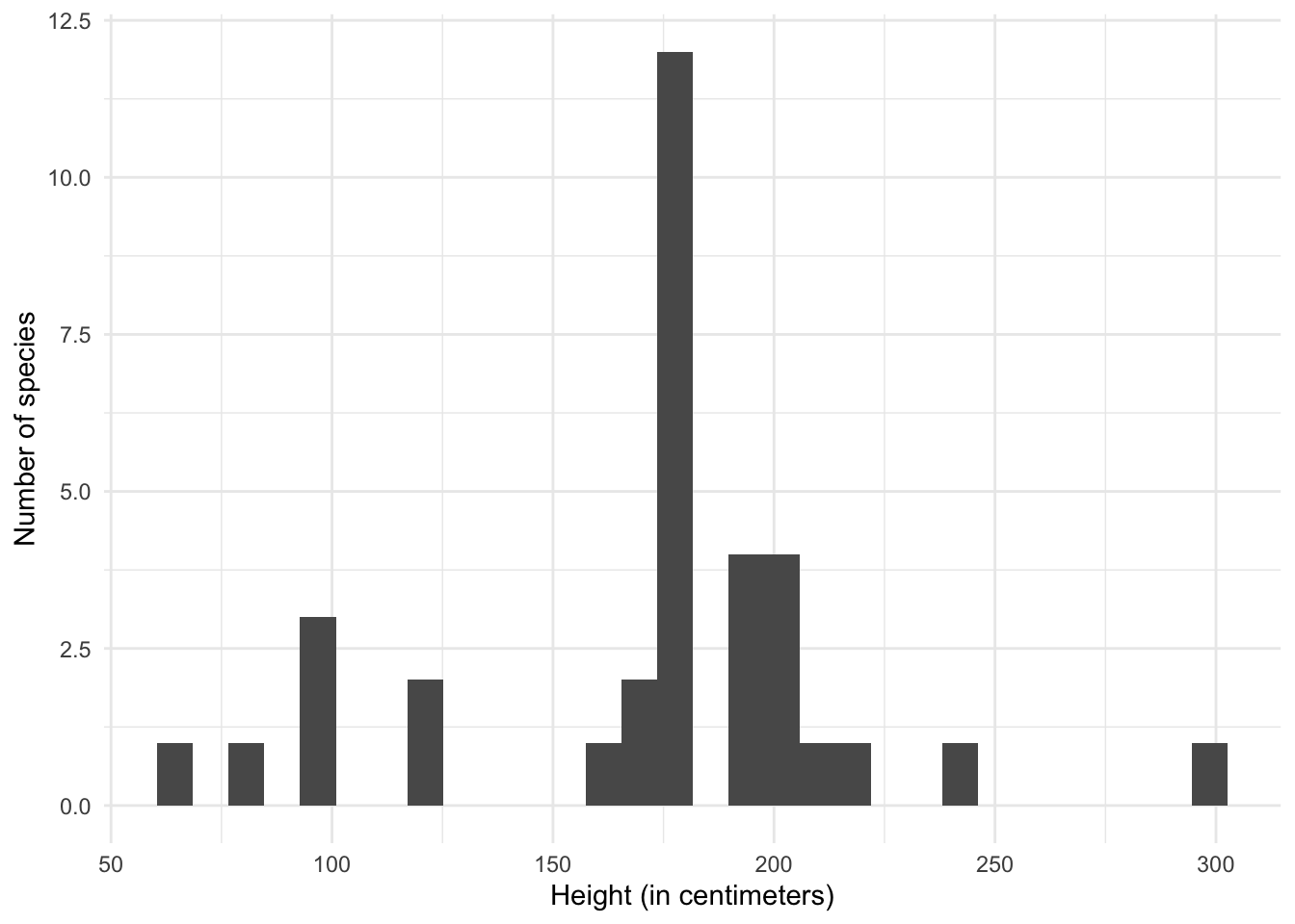

Generate a bar chart showing the number of film appearances made by each character in sw_people who made at least three film appearances.

Click for the solution

Each element of sw_people contains one character. The films element within each character is a character vector containing one value for each film in which the character appeared. This required two separate unnest_*() operations to get the data in the proper form.

# unnest the data
sw_people_df <- tibble(sw_people) %>%
  unnest_wider(sw_people) %>%
  unnest_longer(films)
sw_people_df

## # A tibble: 173 × 16
##    name        height mass  hair_…¹ skin_…² eye_c…³ birth…⁴ gender homew…⁵ films
##    <chr>       <chr>  <chr> <chr>   <chr>   <chr>   <chr>   <chr>  <chr>   <chr>
##  1 Luke Skywa… 172    77    blond   fair    blue    19BBY   male   http:/… http…
##  2 Luke Skywa… 172    77    blond   fair    blue    19BBY   male   http:/… http…
##  3 Luke Skywa… 172    77    blond   fair    blue    19BBY   male   http:/… http…
##  4 Luke Skywa… 172    77    blond   fair    blue    19BBY   male   http:/… http…
##  5 Luke Skywa… 172    77    blond   fair    blue    19BBY   male   http:/… http…
##  6 C-3PO       167    75    n/a     gold    yellow  112BBY  n/a    http:/… http…
##  7 C-3PO       167    75    n/a     gold    yellow  112BBY  n/a    http:/… http…
##  8 C-3PO       167    75    n/a     gold    yellow  112BBY  n/a    http:/… http…
##  9 C-3PO       167    75    n/a     gold    yellow  112BBY  n/a    http:/… http…
## 10 C-3PO       167    75    n/a     gold    yellow  112BBY  n/a    http:/… http…
## # … with 163 more rows, 6 more variables: species <chr>, vehicles <list>,
## #   starships <list>, created <chr>, edited <chr>, url <chr>, and abbreviated
## #   variable names ¹hair_color, ²skin_color, ³eye_color, ⁴birth_year,
## #   ⁵homeworld
## # ℹ Use `print(n = ...)` to see more rows, and `colnames()` to see all variable names

# summarize the data frame and graph the bar chart
sw_people_df %>%
  count(name) %>%
  filter(n >= 3) %>%
  ggplot(mapping = aes(x = fct_reorder(.f = name, .x = n), y = n)) +
  geom_col() +
  coord_flip() +
  labs(
    title = "Number of appearances in the Star Wars cinematic universe",
    subtitle = "As of December 31, 2015",
    x = NULL,
    y = "Number of film appearances"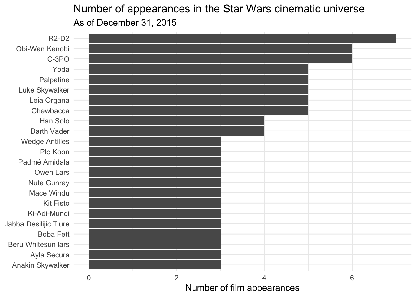
  )

Acknowledgments

Examples and data files drawn from Jenny Bryan’s purrr tutorial
Examples and data files also drawn from the rectangling vignette in tidyr.

Session Info

sessioninfo::session_info()

## ─ Session info ───────────────────────────────────────────────────────────────
##  setting  value
##  version  R version 4.2.1 (2022-06-23)
##  os       macOS Monterey 12.3
##  system   aarch64, darwin20
##  ui       X11
##  language (EN)
##  collate  en_US.UTF-8
##  ctype    en_US.UTF-8
##  tz       America/New_York
##  date     2022-08-22
##  pandoc   2.18 @ /Applications/RStudio.app/Contents/MacOS/quarto/bin/tools/ (via rmarkdown)
## 
## ─ Packages ───────────────────────────────────────────────────────────────────
##  package       * version    date (UTC) lib source
##  assertthat      0.2.1      2019-03-21 [2] CRAN (R 4.2.0)
##  backports       1.4.1      2021-12-13 [2] CRAN (R 4.2.0)
##  blogdown        1.10       2022-05-10 [2] CRAN (R 4.2.0)
##  bookdown        0.27       2022-06-14 [2] CRAN (R 4.2.0)
##  broom           1.0.0      2022-07-01 [2] CRAN (R 4.2.0)
##  bslib           0.4.0      2022-07-16 [2] CRAN (R 4.2.0)
##  cachem          1.0.6      2021-08-19 [2] CRAN (R 4.2.0)
##  cellranger      1.1.0      2016-07-27 [2] CRAN (R 4.2.0)
##  cli             3.3.0      2022-04-25 [2] CRAN (R 4.2.0)
##  colorspace      2.0-3      2022-02-21 [2] CRAN (R 4.2.0)
##  crayon          1.5.1      2022-03-26 [2] CRAN (R 4.2.0)
##  DBI             1.1.3      2022-06-18 [2] CRAN (R 4.2.0)
##  dbplyr          2.2.1      2022-06-27 [2] CRAN (R 4.2.0)
##  digest          0.6.29     2021-12-01 [2] CRAN (R 4.2.0)
##  dplyr         * 1.0.9      2022-04-28 [2] CRAN (R 4.2.0)
##  ellipsis        0.3.2      2021-04-29 [2] CRAN (R 4.2.0)
##  evaluate        0.16       2022-08-09 [1] CRAN (R 4.2.1)
##  fansi           1.0.3      2022-03-24 [2] CRAN (R 4.2.0)
##  fastmap         1.1.0      2021-01-25 [2] CRAN (R 4.2.0)
##  forcats       * 0.5.1      2021-01-27 [2] CRAN (R 4.2.0)
##  fs              1.5.2      2021-12-08 [2] CRAN (R 4.2.0)
##  gargle          1.2.0      2021-07-02 [2] CRAN (R 4.2.0)
##  generics        0.1.3      2022-07-05 [2] CRAN (R 4.2.0)
##  ggplot2       * 3.3.6      2022-05-03 [2] CRAN (R 4.2.0)
##  glue            1.6.2      2022-02-24 [2] CRAN (R 4.2.0)
##  googledrive     2.0.0      2021-07-08 [2] CRAN (R 4.2.0)
##  googlesheets4   1.0.0      2021-07-21 [2] CRAN (R 4.2.0)
##  gtable          0.3.0      2019-03-25 [2] CRAN (R 4.2.0)
##  haven           2.5.0      2022-04-15 [2] CRAN (R 4.2.0)
##  here            1.0.1      2020-12-13 [2] CRAN (R 4.2.0)
##  hms             1.1.1      2021-09-26 [2] CRAN (R 4.2.0)
##  htmltools       0.5.3      2022-07-18 [2] CRAN (R 4.2.0)
##  httr          * 1.4.3      2022-05-04 [2] CRAN (R 4.2.0)
##  jquerylib       0.1.4      2021-04-26 [2] CRAN (R 4.2.0)
##  jsonlite        1.8.0      2022-02-22 [2] CRAN (R 4.2.0)
##  knitr           1.39       2022-04-26 [2] CRAN (R 4.2.0)
##  lifecycle       1.0.1      2021-09-24 [2] CRAN (R 4.2.0)
##  lubridate       1.8.0      2021-10-07 [2] CRAN (R 4.2.0)
##  magrittr        2.0.3      2022-03-30 [2] CRAN (R 4.2.0)
##  modelr          0.1.8      2020-05-19 [2] CRAN (R 4.2.0)
##  munsell         0.5.0      2018-06-12 [2] CRAN (R 4.2.0)
##  pillar          1.8.0      2022-07-18 [2] CRAN (R 4.2.0)
##  pkgconfig       2.0.3      2019-09-22 [2] CRAN (R 4.2.0)
##  purrr         * 0.3.4      2020-04-17 [2] CRAN (R 4.2.0)
##  R6              2.5.1      2021-08-19 [2] CRAN (R 4.2.0)
##  readr         * 2.1.2      2022-01-30 [2] CRAN (R 4.2.0)
##  readxl          1.4.0      2022-03-28 [2] CRAN (R 4.2.0)
##  reprex          2.0.1.9000 2022-08-10 [1] Github (tidyverse/reprex@6d3ad07)
##  repurrrsive   * 1.0.0      2019-07-15 [2] CRAN (R 4.2.0)
##  rlang           1.0.4      2022-07-12 [2] CRAN (R 4.2.0)
##  rmarkdown       2.14       2022-04-25 [2] CRAN (R 4.2.0)
##  rprojroot       2.0.3      2022-04-02 [2] CRAN (R 4.2.0)
##  rstudioapi      0.13       2020-11-12 [2] CRAN (R 4.2.0)
##  rvest           1.0.2      2021-10-16 [2] CRAN (R 4.2.0)
##  sass            0.4.2      2022-07-16 [2] CRAN (R 4.2.0)
##  scales          1.2.0      2022-04-13 [2] CRAN (R 4.2.0)
##  sessioninfo     1.2.2      2021-12-06 [2] CRAN (R 4.2.0)
##  stringi         1.7.8      2022-07-11 [2] CRAN (R 4.2.0)
##  stringr       * 1.4.0      2019-02-10 [2] CRAN (R 4.2.0)
##  tibble        * 3.1.8      2022-07-22 [2] CRAN (R 4.2.0)
##  tidyr         * 1.2.0      2022-02-01 [2] CRAN (R 4.2.0)
##  tidyselect      1.1.2      2022-02-21 [2] CRAN (R 4.2.0)
##  tidyverse     * 1.3.2      2022-07-18 [2] CRAN (R 4.2.0)
##  tzdb            0.3.0      2022-03-28 [2] CRAN (R 4.2.0)
##  utf8            1.2.2      2021-07-24 [2] CRAN (R 4.2.0)
##  vctrs           0.4.1      2022-04-13 [2] CRAN (R 4.2.0)
##  withr           2.5.0      2022-03-03 [2] CRAN (R 4.2.0)
##  xfun            0.31       2022-05-10 [1] CRAN (R 4.2.0)
##  xml2            1.3.3      2021-11-30 [2] CRAN (R 4.2.0)
##  yaml            2.3.5      2022-02-21 [2] CRAN (R 4.2.0)
## 
##  [1] /Users/soltoffbc/Library/R/arm64/4.2/library
##  [2] /Library/Frameworks/R.framework/Versions/4.2-arm64/Resources/library
## 
## ──────────────────────────────────────────────────────────────────────────────

Last updated on Mar 1, 2019