Using APIs to get data
library(tidyverse)
library(forcats)
library(broom)
library(wbstats)
library(wordcloud)
library(tidytext)
library(viridis)

set.seed(1234)
theme_set(theme_minimal())
There are many ways to obtain data from the Internet. Four major categories are:
- click-and-download on the internet as a “flat” file, such as .csv, .xls
- install-and-play an API for which someone has written a handy R package
- API-query published with an unwrapped API
- Scraping implicit in an html website
Click-and-Download
In the simplest case, the data you need is already on the internet in a tabular format. There are a couple of strategies here:
- Use
read.csvorreadr::read_csvto read the data straight into R - Use the
downloaderpackage orcurlfrom the shell to download the file and store a local copy, then useread_csvor something similar to read the data into R- Even if the file disappears from the internet, you have a local copy cached
Even in this instance, files may need cleaning and transformation when you bring them into R.
Data supplied on the web - APIs
Many times, the data that you want is not already organized into one or a few tables that you can read directly into R. More frequently, you find this data is given in the form of an API. Application Programming Interfaces (APIs) are descriptions of the kind of requests that can be made of a certain piece of software, and descriptions of the kind of answers that are returned. Many sources of data - databases, websites, services - have made all (or part) of their data available via APIs over the internet. Computer programs (“clients”) can make requests of the server, and the server will respond by sending data (or an error message). This client can be many kinds of other programs or websites, including R running from your laptop.
Some basic terminology
- Representational State Transfer (REST) - these allow us to query databases using URLs, just like you would construct a URL to view a web page.
- Uniform Resource Location (URL) - a string of characters that uses the Hypertext Transfer Protocol (HTTP) and points to a data resource. On the world wide web this is typically a file written in Hypertext Markup Language (HTML). Here, it will return a file containing a subset of a database.
- HTTP methods/verbs
- GET: fetch an existing resource. The URL contains all the necessary information the server needs to locate and return the resource.
- POST: create a new resource. POST requests usually carry a payload that specifies the data for the new resource.
- PUT: update an existing resource. The payload may contain the updated data for the resource.
- DELETE: delete an existing resource.
- The most common method you will use for an API is GET.
How Do GET Requests Work?
A Web Browsing Example {-}
As you might suspect from the example above, surfing the web is basically equivalent to sending a bunch of GET requests to different servers and asking for different files written in HTML.
Suppose, for instance, you wanted to look something up on Wikipedia. The first step would be to open your web browser and type in http://www.wikipedia.org. Once you hit return, you would see the page below.
Several different processes occurred, however, between hitting “return” and the page finally being rendered. In order:
- The web browser took the entered character string, used the command-line tool “Curl” to write a properly formatted HTTP GET request, and submitted it to the server that hosts the Wikipedia homepage.
- After receiving this request, the server sent an HTTP response, from which Curl extracted the HTML code for the page (partially shown below).
- The raw HTML code was parsed and then executed by the web browser, rendering the page as seen in the window.
## No encoding supplied: defaulting to UTF-8.
## [1] "<!DOCTYPE html>\n<html lang=\"en\" class=\"no-js\">\n<head>\n<meta charset=\"utf-8\">\n<title>Wikipedia</title>\n<meta name=\"description\" content=\"Wikipedia is a free online encyclopedia, created and edited by volunteers around the world and hosted by the Wikimedia Foundation.\">\n<script>\ndocument.documentElement.className = document.documentElement.className.replace( /(^|\\s)no-js(\\s|$)/, \"$1js-enabled$2\" );\n</script>\n<meta name=\"viewport\" content=\"initial-scale=1,user-scalable=yes\">\n<link rel=\"apple-touch-icon\" href=\"/static/apple-touch/wikipedia.png\">\n<link rel=\"shortcut icon\" href=\"/static/favicon/wikipedia.ico\">\n<link rel=\"license\" href=\"//creativecommons.org/licenses/by-sa/3.0/\">\n<style>\n.sprite{background-image:linear-gradient(transparent,transparent),url(portal/wikipedia.org/assets/img/sprite-e99844f6.svg);background-repeat:no-repeat;display:inline-block;vertical-align:middle}.svg-Commons-logo_sister{background-position:0 0;width:47px;height:47px}.svg-MediaWiki-logo_sister{background-positi"
Web Browsing as a Template for RESTful Database Querying
The process of web browsing described above is a close analogue for the process of database querying via RESTful APIs, with only a few adjustments:
While the Curl tool will still be used to send HTML GET requests to the servers hosting our databases of interest, the character string that we supply to Curl must be constructed so that the resulting request can be interpreted and successfully acted upon by the server. In particular, it is likely that the character string must encode search terms and/or filtering parameters, as well as one or more authentication codes. While the terms are often similar across APIs, most are API-specific.
Unlike with web browsing, the content of the server’s response that is extracted by Curl is unlikely to be HTML code. Rather, it will likely be raw text response that can be parsed into one of a few file formats commonly used for data storage. The usual suspects include
.csv,.xml, and.jsonfiles.Whereas the web browser capably parsed and executed the HTML code, one or more facilities in R, Python, or other programming languages will be necessary for parsing the server response and converting it into a format for local storage (e.g., matrices, dataframes, databases, lists, etc.).
Install and play packages
Many common web services and APIs have been “wrapped”, i.e. R functions have been written around them which send your query to the server and format the response.
Why do we want this?
- provenance
- reproducible
- updating
- ease
- scaling
Obtaining World Bank indicators
The World Bank contains a rich and detailed set of socioeconomic indicators spanning several decades and dozens of topics. Their data is available for bulk download as CSV files from their website; you previously practiced importing and wrangling this data for all countries. However as you noted in that assignment, frequently you only need to obtain a handful of indicators or a subset of countries.
To provide more granular access to this information, the World Bank provides a RESTful API for querying and obtaining a portion of their database programmatically. The wbstats implements this API in R to allow for relatively easy access to the API and return the results in a tidy data frame.
Finding available data with wb_cachelist
wb_cachelist contains a snapshot of available countries, indicators, and other relevant information obtainable through the WB API.
library(wbstats)

str(wb_cachelist, max.level = 1)
## List of 8
##  $ countries    : tibble [304 × 18] (S3: tbl_df/tbl/data.frame)
##  $ indicators   : tibble [16,649 × 8] (S3: tbl_df/tbl/data.frame)
##  $ sources      : tibble [63 × 9] (S3: tbl_df/tbl/data.frame)
##  $ topics       : tibble [21 × 3] (S3: tbl_df/tbl/data.frame)
##  $ regions      : tibble [48 × 4] (S3: tbl_df/tbl/data.frame)
##  $ income_levels: tibble [7 × 3] (S3: tbl_df/tbl/data.frame)
##  $ lending_types: tibble [4 × 3] (S3: tbl_df/tbl/data.frame)
##  $ languages    : tibble [23 × 3] (S3: tbl_df/tbl/data.frame)
glimpse(wb_cachelist$countries)
## Rows: 304
## Columns: 18
## $ iso3c              <chr> "ABW", "AFG", "AFR", "AGO", "ALB", "AND", "ANR", "A…
## $ iso2c              <chr> "AW", "AF", "A9", "AO", "AL", "AD", "L5", "1A", "AE…
## $ country            <chr> "Aruba", "Afghanistan", "Africa", "Angola", "Albani…
## $ capital_city       <chr> "Oranjestad", "Kabul", NA, "Luanda", "Tirane", "And…
## $ longitude          <dbl> -70.01670, 69.17610, NA, 13.24200, 19.81720, 1.5218…
## $ latitude           <dbl> 12.51670, 34.52280, NA, -8.81155, 41.33170, 42.5075…
## $ region_iso3c       <chr> "LCN", "SAS", NA, "SSF", "ECS", "ECS", NA, NA, "MEA…
## $ region_iso2c       <chr> "ZJ", "8S", NA, "ZG", "Z7", "Z7", NA, NA, "ZQ", "ZJ…
## $ region             <chr> "Latin America & Caribbean", "South Asia", "Aggrega…
## $ admin_region_iso3c <chr> NA, "SAS", NA, "SSA", "ECA", NA, NA, NA, NA, "LAC",…
## $ admin_region_iso2c <chr> NA, "8S", NA, "ZF", "7E", NA, NA, NA, NA, "XJ", "7E…
## $ admin_region       <chr> NA, "South Asia", NA, "Sub-Saharan Africa (excludin…
## $ income_level_iso3c <chr> "HIC", "LIC", NA, "LMC", "UMC", "HIC", NA, NA, "HIC…
## $ income_level_iso2c <chr> "XD", "XM", NA, "XN", "XT", "XD", NA, NA, "XD", "XT…
## $ income_level       <chr> "High income", "Low income", "Aggregates", "Lower m…
## $ lending_type_iso3c <chr> "LNX", "IDX", NA, "IBD", "IBD", "LNX", NA, NA, "LNX…
## $ lending_type_iso2c <chr> "XX", "XI", NA, "XF", "XF", "XX", NA, NA, "XX", "XF…
## $ lending_type       <chr> "Not classified", "IDA", "Aggregates", "IBRD", "IBR…
Search available data with wb_search()
wb_search() searches through the wb_cachelist$indicators data frame to find indicators that match the search pattern.1
wb_search("unemployment")
## # A tibble: 61 × 3
## indicator_id indicator indic…¹
## <chr> <chr> <chr>
## 1 fin37.t.a Received government transfers in the past year (% age 1… The pe…
## 2 fin37.t.a.1 Received government transfers in the past year, male (… The pe…
## 3 fin37.t.a.10 Received government transfers in the past year, in labo… The pe…
## 4 fin37.t.a.11 Received government transfers in the past year, out of … The pe…
## 5 fin37.t.a.2 Received government transfers in the past year, female … The pe…
## 6 fin37.t.a.3 Received government transfers in the past year, young a… The pe…
## 7 fin37.t.a.4 Received government transfers in the past year, older a… The pe…
## 8 fin37.t.a.5 Received government transfers in the past year, primary… The pe…
## 9 fin37.t.a.6 Received government transfers in the past year, seconda… The pe…
## 10 fin37.t.a.7 Received government transfers in the past year, income,… The pe…
## # … with 51 more rows, and abbreviated variable name ¹indicator_desc
## # ℹ Use `print(n = ...)` to see more rows
wb_search("labor force")
## # A tibble: 245 × 3
## indicator_id indicator indic…¹
## <chr> <chr> <chr>
## 1 9.0.Employee.All Employees (%) Share …
## 2 9.0.Employee.B40 Employees-Bottom 40 Percent (%) Share …
## 3 9.0.Employee.T60 Employees-Top 60 Percent (%) Share …
## 4 9.0.Employer.All Employers (%) Share …
## 5 9.0.Employer.B40 Employers-Bottom 40 Percent (%) Share …
## 6 9.0.Employer.T60 Employers-Top 60 Percent (%) Share …
## 7 9.0.Labor.All Labor Force Participation Rate (%) Share …
## 8 9.0.Labor.B40 Labor Force Participation Rate (%)-Bottom 40 Percent Share …
## 9 9.0.Labor.T60 Labor Force Participation Rate (%)-Top 60 Percent Share …
## 10 9.0.SelfEmp.All Self-Employed (%) Share …
## # … with 235 more rows, and abbreviated variable name ¹indicator_desc
## # ℹ Use `print(n = ...)` to see more rows
wb_search("labor force", fields = "indicator") # limit search to just the indicator name
## # A tibble: 176 × 3
## indicator_id indicator indic…¹
## <chr> <chr> <chr>
## 1 9.0.Labor.All Labor Force Participation Rate (%) Share …
## 2 9.0.Labor.B40 Labor Force Participation Rate (%)-Bottom 40 Percent Share …
## 3 9.0.Labor.T60 Labor Force Participation Rate (%)-Top 60 Percent Share …
## 4 9.1.Labor.All Labor Force Participation Rate (%), Male Share …
## 5 9.1.Labor.B40 Labor Force Participation Rate (%)-Bottom 40 Percent,… Share …
## 6 9.1.Labor.T60 Labor Force Participation Rate (%)-Top 60 Percent, Ma… Share …
## 7 9.2.Labor.All Labor Force Participation Rate (%), Female Share …
## 8 9.2.Labor.B40 Labor Force Participation Rate (%)-Bottom 40 Percent,… Share …
## 9 9.2.Labor.T60 Labor Force Participation Rate (%)-Top 60 Percent, Fe… Share …
## 10 account.t.d.10 Account, in labor force (% age 15+) The pe…
## # … with 166 more rows, and abbreviated variable name ¹indicator_desc
## # ℹ Use `print(n = ...)` to see more rows
Downloading data with wb_data()
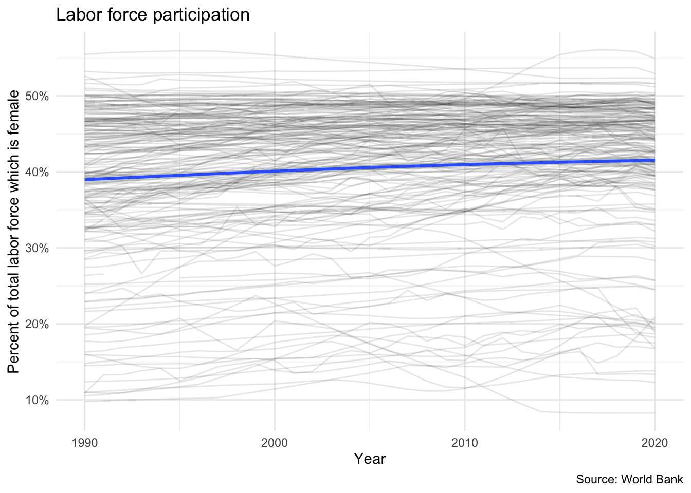
Once you have the set of indicators you would like to obtain, you can use the wb_data() function to generate the API query and download the results. Let’s say we want to obtain information on the percent of females participating in the labor force. The indicator ID is SL.TLF.TOTL.FE.ZS. We can download the indicator for all countries from 1990-2020 using:
female_labor <- wb_data(
  indicator = "SL.TLF.TOTL.FE.ZS",
  start_date = 1990,
  end_date = 2020
)
female_labor
## # A tibble: 6,727 × 9
## iso2c iso3c country date SL.TLF.TOTL.FE.ZS unit obs_st…¹ footn…² last_upd…³
## <chr> <chr> <chr> <dbl> <dbl> <chr> <chr> <chr> <date>
## 1 AW ABW Aruba 1990 NA <NA> <NA> <NA> 2022-07-20
## 2 AW ABW Aruba 1991 NA <NA> <NA> <NA> 2022-07-20
## 3 AW ABW Aruba 1992 NA <NA> <NA> <NA> 2022-07-20
## 4 AW ABW Aruba 1993 NA <NA> <NA> <NA> 2022-07-20
## 5 AW ABW Aruba 1994 NA <NA> <NA> <NA> 2022-07-20
## 6 AW ABW Aruba 1995 NA <NA> <NA> <NA> 2022-07-20
## 7 AW ABW Aruba 1996 NA <NA> <NA> <NA> 2022-07-20
## 8 AW ABW Aruba 1997 NA <NA> <NA> <NA> 2022-07-20
## 9 AW ABW Aruba 1998 NA <NA> <NA> <NA> 2022-07-20
## 10 AW ABW Aruba 1999 NA <NA> <NA> <NA> 2022-07-20
## # … with 6,717 more rows, and abbreviated variable names ¹obs_status,
## # ²footnote, ³last_updated
## # ℹ Use `print(n = ...)` to see more rows
Note the column containing our indicator uses the indicator ID as its name. This is rather unintuitive, so we can adjust it directly in the function.
female_labor <- wb_data(
  indicator = c("fem_lab_part" = "SL.TLF.TOTL.FE.ZS"),
  start_date = 1990,
  end_date = 2020
)
female_labor
## # A tibble: 6,727 × 9
##    iso2c iso3c country  date fem_lab_part unit  obs_status footnote last_updated
##    <chr> <chr> <chr>   <dbl>        <dbl> <chr> <chr>      <chr>    <date>
##  1 AW    ABW   Aruba    1990           NA <NA>  <NA>       <NA>     2022-07-20
##  2 AW    ABW   Aruba    1991           NA <NA>  <NA>       <NA>     2022-07-20
##  3 AW    ABW   Aruba    1992           NA <NA>  <NA>       <NA>     2022-07-20
##  4 AW    ABW   Aruba    1993           NA <NA>  <NA>       <NA>     2022-07-20
##  5 AW    ABW   Aruba    1994           NA <NA>  <NA>       <NA>     2022-07-20
##  6 AW    ABW   Aruba    1995           NA <NA>  <NA>       <NA>     2022-07-20
##  7 AW    ABW   Aruba    1996           NA <NA>  <NA>       <NA>     2022-07-20
##  8 AW    ABW   Aruba    1997           NA <NA>  <NA>       <NA>     2022-07-20
##  9 AW    ABW   Aruba    1998           NA <NA>  <NA>       <NA>     2022-07-20
## 10 AW    ABW   Aruba    1999           NA <NA>  <NA>       <NA>     2022-07-20
## # … with 6,717 more rows
## # ℹ Use `print(n = ...)` to see more rows
ggplot(data = female_labor, mapping = aes(x = date, y = fem_lab_part)) +
  geom_line(mapping = aes(group = country), alpha = .1) +
  geom_smooth() +
  scale_y_continuous(labels = scales::percent_format(scale = 1)) +
  labs(
    title = "Labor force participation",
    x = "Year",
    y = "Percent of total labor force which is female",
    caption = "Source: World Bank"
  )
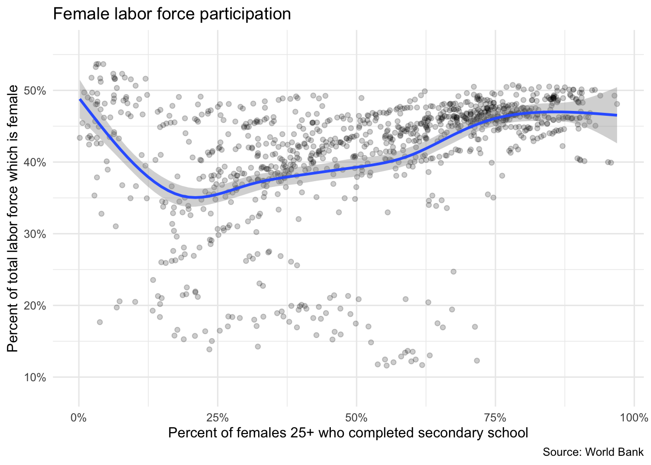
By default, wb_data() returns queries as data frames in a wide format. So if we request multiple indicators, each indicator will be stored in its own column.
female_vars <- wb_data(
  indicator = c(
    "fem_lab_part" = "SL.TLF.TOTL.FE.ZS",
    "fem_educ_sec" = "SE.SEC.CUAT.UP.FE.ZS"
  ),
  start_date = 1990,
  end_date = 2020
)

ggplot(data = female_vars, mapping = aes(x = fem_educ_sec, y = fem_lab_part)) +
  geom_point(alpha = .2) +
  geom_smooth() +
  scale_x_continuous(labels = scales::percent_format(scale = 1)) +
  scale_y_continuous(labels = scales::percent_format(scale = 1)) +
  labs(
    title = "Female labor force participation",
    x = "Percent of females 25+ who completed secondary school",
    y = "Percent of total labor force which is female",
    caption = "Source: World Bank"
  )
Searching geographic info: geonames
# install.packages(geonames)
library(geonames)
API authentication
Many APIs require you to register for access. This allows them to track which users are submitting queries and manage demand - if you submit too many queries too quickly, you might be rate-limited and your requests de-prioritized or blocked. Always check the API access policy of the web site to determine what these limits are.
There are a few things we need to do to be able to use this package to access the geonames API:
- Go to the geonames site and register an account.
- Click here to enable the free web service
- Tell R your geonames username. You could run the line
options(geonamesUsername = "my_user_name")
in R. However this is insecure. We don’t want to risk committing this line and pushing it to our public GitHub page! Instead, you should create a file in the same place as your .Rproj file. To do that, run the following command from the R console:
usethis::edit_r_profile(scope = "project")
This will create a special file called .Rprofile in the same directory as your .Rproj file (assuming you are working in an R project). The file should open automatically in your RStudio script editor. Add
options(geonamesUsername = "my_user_name")
to that file, replacing my_user_name with your Geonames username.
Important
- Make sure your
.Rprofileends with a blank line - Make sure
.Rprofileis included in your.gitignorefile, otherwise it will be synced with Github - Restart RStudio after modifying
.Rprofilein order to load any new keys into memory - Spelling is important when you set the option in your
.Rprofile - You can do a similar process for an arbitrary package or key. For example:
# in .Rprofile
options(this_is_my_key = "XXXX")

# later, in the R script:
key <- getOption("this_is_my_key")
This is a simple means to keep your keys private, especially if you are sharing the same authentication across several projects. Remember that using .Rprofile makes your code un-reproducible. In this case, that is exactly what we want!
Using Geonames
What can we do? Get access to lots of geographical information via the various “web services”
countryInfo <- GNcountryInfo()
countryInfo %>%
  as_tibble() %>%
  glimpse()
## Rows: 250
## Columns: 18
## $ continent        <chr> "EU", "AS", "AS", "NA", "NA", "EU", "AS", "AF", "AN",…
## $ capital          <chr> "Andorra la Vella", "Abu Dhabi", "Kabul", "Saint John…
## $ languages        <chr> "ca", "ar-AE,fa,en,hi,ur", "fa-AF,ps,uz-AF,tk", "en-A…
## $ geonameId        <chr> "3041565", "290557", "1149361", "3576396", "3573511",…
## $ south            <chr> "42.428743001", "22.6315119400001", "29.3770645357176…
## $ isoAlpha3        <chr> "AND", "ARE", "AFG", "ATG", "AIA", "ALB", "ARM", "AGO…
## $ north            <chr> "42.655765", "26.0693916590001", "38.4907920755748", …
## $ fipsCode         <chr> "AN", "AE", "AF", "AC", "AV", "AL", "AM", "AO", "AY",…
## $ population       <chr> "77006", "9630959", "37172386", "96286", "13254", "28…
## $ east             <chr> "1.78657600000003", "56.381222289", "74.8894511481168…
## $ isoNumeric       <chr> "020", "784", "004", "028", "660", "008", "051", "024…
## $ areaInSqKm       <chr> "468.0", "82880.0", "647500.0", "443.0", "102.0", "28…
## $ countryCode      <chr> "AD", "AE", "AF", "AG", "AI", "AL", "AM", "AO", "AQ",…
## $ west             <chr> "1.41376000100007", "51.5904085340001", "60.472083397…
## $ countryName      <chr> "Principality of Andorra", "United Arab Emirates", "I…
## $ postalCodeFormat <chr> "AD###", "", "", "", "", "####", "######", "", "", "@…
## $ continentName    <chr> "Europe", "Asia", "Asia", "North America", "North Ame…
## $ currencyCode     <chr> "EUR", "AED", "AFN", "XCD", "XCD", "ALL", "AMD", "AOA…
This country info dataset is very helpful for accessing the rest of the data, because it gives us the standardized codes for country and language.
The Manifesto Project: manifestoR
The Manifesto Project collects and organizes political party manifestos from around the world. It currently covers over 1000 parties from 1945 until today in over 50 countries on five continents. We can use the manifestoR package to access the API and download those manifestos for analysis in R.
Load library and set API key
Accessing data from the Manifesto Project API requires an authentication key. You can create an account and key here. Here I store my key in .Rprofile and retrieve it using mp_setapikey().
library(manifestoR)

# retrieve API key stored in .Rprofile
mp_setapikey(key = getOption("manifesto_key"))
Retrieve the database
(mpds <- mp_maindataset())
## Connecting to Manifesto Project DB API...
## Connecting to Manifesto Project DB API... corpus version: 2021-1
## # A tibble: 4,739 × 174
##    country countryname oecdmem…¹ eumem…² edate        date party party…³ party…⁴
##      <dbl> <chr>           <dbl>   <dbl> <date>      <dbl> <dbl> <chr>   <chr>
##  1      11 Sweden              0       0 1944-09-17 194409 11220 Commun… "SKP"
##  2      11 Sweden              0       0 1944-09-17 194409 11320 Social… "SAP"
##  3      11 Sweden              0       0 1944-09-17 194409 11420 People… "FP"
##  4      11 Sweden              0       0 1944-09-17 194409 11620 Right … ""
##  5      11 Sweden              0       0 1944-09-17 194409 11810 Agrari… ""
##  6      11 Sweden              0       0 1948-09-19 194809 11220 Commun… "SKP"
##  7      11 Sweden              0       0 1948-09-19 194809 11320 Social… "SAP"
##  8      11 Sweden              0       0 1948-09-19 194809 11420 People… "FP"
##  9      11 Sweden              0       0 1948-09-19 194809 11620 Right … ""
## 10      11 Sweden              0       0 1948-09-19 194809 11810 Agrari… ""
## # … with 4,729 more rows, 165 more variables: parfam <dbl>, coderid <dbl>,
## #   manual <dbl>, coderyear <dbl>, testresult <dbl>, testeditsim <dbl>,
## #   pervote <dbl>, voteest <dbl>, presvote <dbl>, absseat <dbl>,
## #   totseats <dbl>, progtype <dbl>, datasetorigin <dbl>, corpusversion <chr>,
## #   total <dbl>, peruncod <dbl>, per101 <dbl>, per102 <dbl>, per103 <dbl>,
## #   per104 <dbl>, per105 <dbl>, per106 <dbl>, per107 <dbl>, per108 <dbl>,
## #   per109 <dbl>, per110 <dbl>, per201 <dbl>, per202 <dbl>, per203 <dbl>, …
## # ℹ Use `print(n = ...)` to see more rows, and `colnames()` to see all variable names
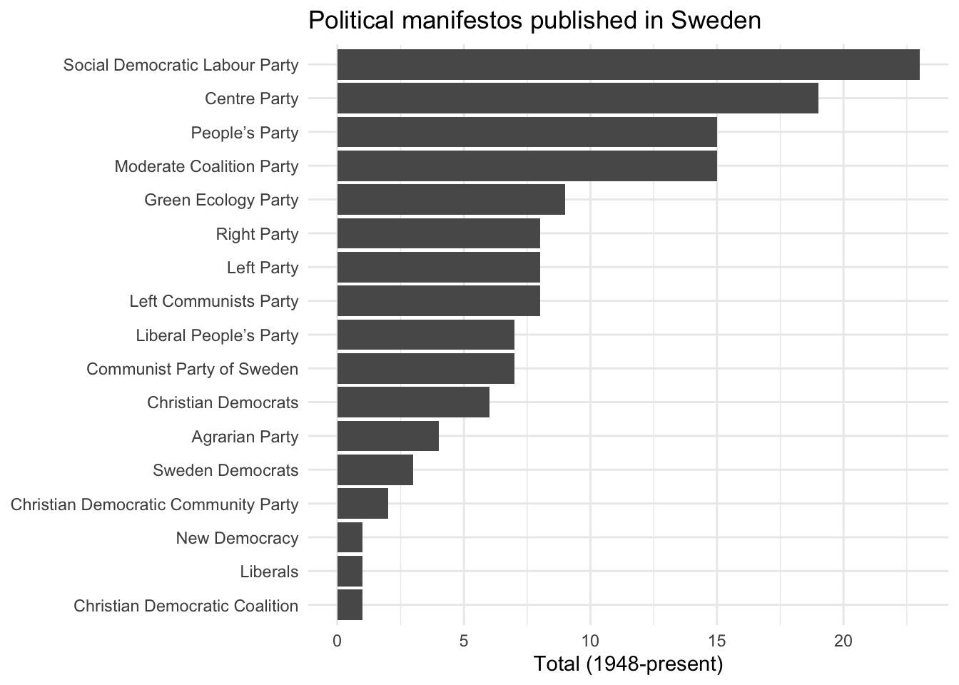
mp_maindataset() includes a data frame describing each manifesto included in the database. You can use this database for some exploratory data analysis. For instance, how many manifestos have been published by each political party in Sweden?
mpds %>%
  filter(countryname == "Sweden") %>%
  count(partyname) %>%
  ggplot(aes(fct_reorder(partyname, n), n)) +
  geom_col() +
  labs(
    title = "Political manifestos published in Sweden",
    x = NULL,
    y = "Total (1948-present)"
  ) +
  coord_flip()
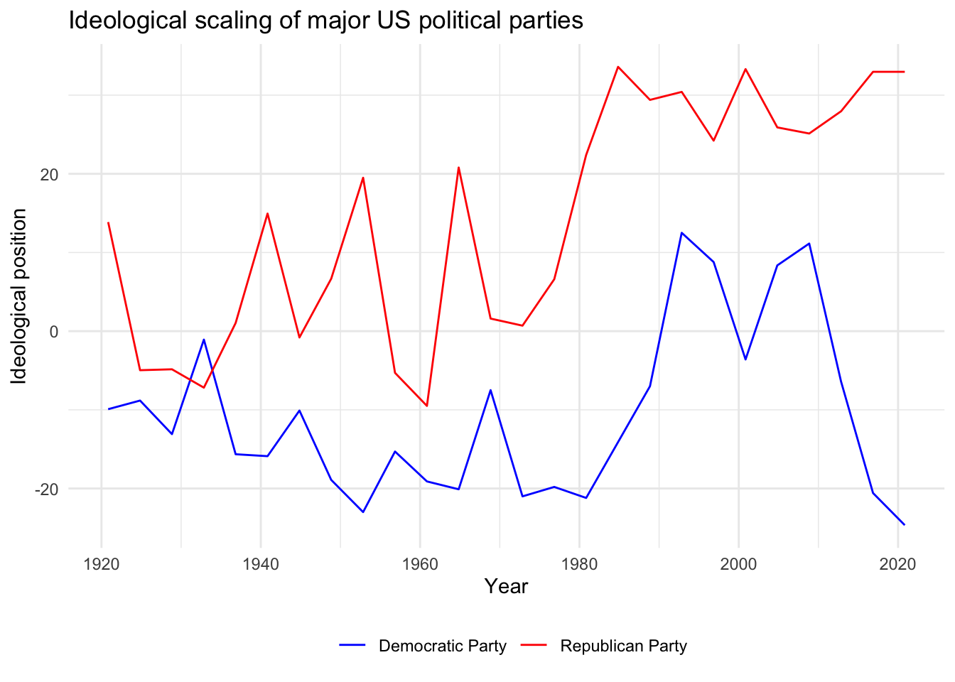
Or we can use scaling functions to identify each party manifesto on an ideological dimension. For example, how have the Democratic and Republican Party manifestos in the United States changed over time?
mpds %>%
  filter(party == 61320 | party == 61620) %>%
  mutate(ideo = mp_scale(.)) %>%
  select(partyname, edate, ideo) %>%
  ggplot(aes(edate, ideo, color = partyname)) +
  geom_line() +
  scale_color_manual(values = c("blue", "red")) +
  labs(
    title = "Ideological scaling of major US political parties",
    x = "Year",
    y = "Ideological position",
    color = NULL
  ) +
  theme(legend.position = "bottom")
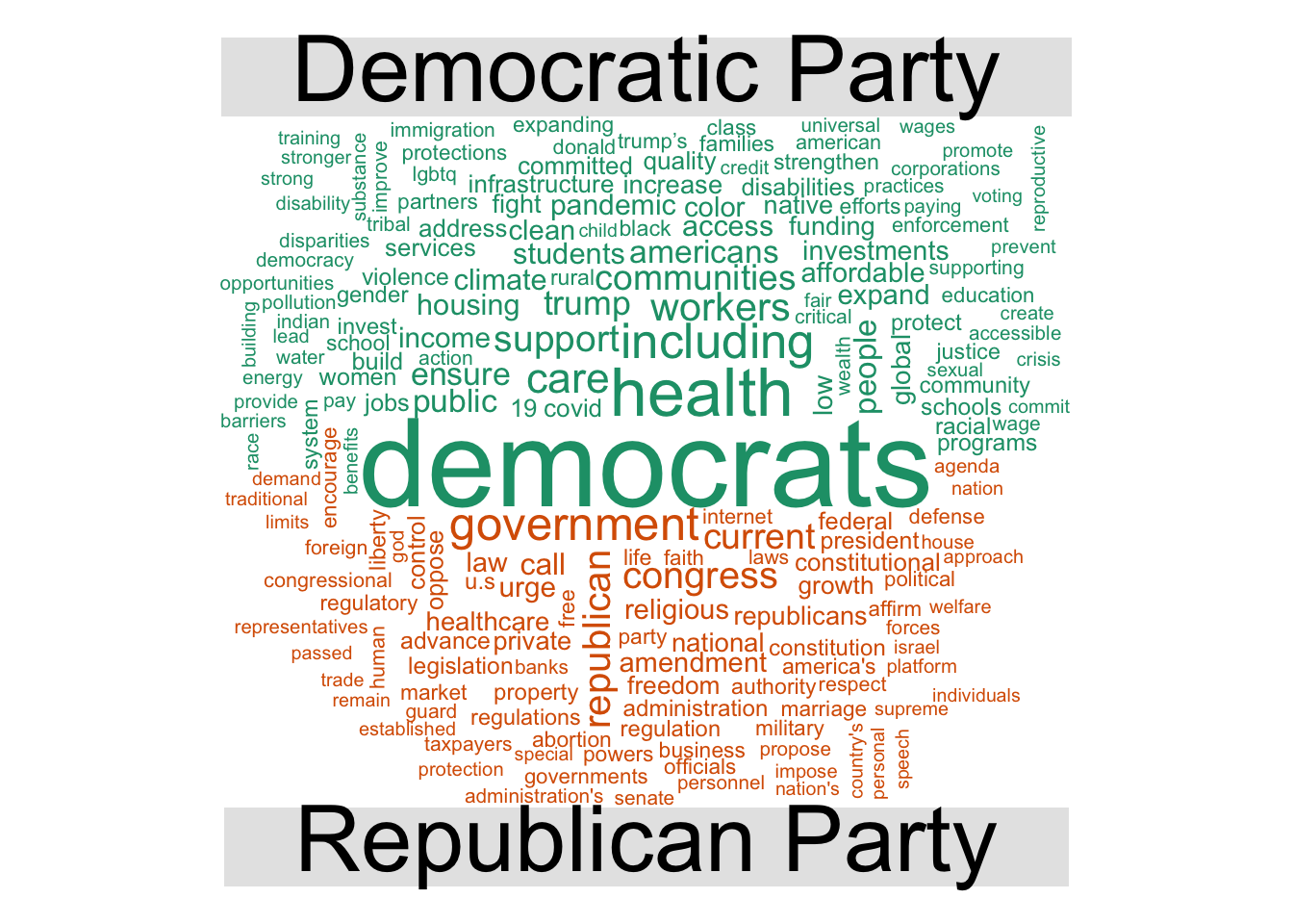
Download manifestos
mp_corpus() can be used to download the original manifestos as full text documents stored as a corpus. Once you obtain the corpus, you can perform text analysis. As an example, let’s compare the most common words in the Democratic and Republican Party manifestos from the 2016 U.S. presidential election:
# download documents
(docs <- mp_corpus(countryname == "United States" & edate > as.Date("2016-01-01")))
## Connecting to Manifesto Project DB API...
## Connecting to Manifesto Project DB API... corpus version: 2021-1
## Connecting to Manifesto Project DB API... corpus version: 2021-1
## Connecting to Manifesto Project DB API... corpus version: 2021-1
## <<ManifestoCorpus>>
## Metadata:  corpus specific: 0, document level (indexed): 0
## Content:  documents: 4
# generate wordcloud of most common terms
docs %>%
  tidy() %>%
  mutate(party = factor(party,
    levels = c(61320, 61620),
    labels = c("Democratic Party", "Republican Party")
  )) %>%
  unnest_tokens(word, text) %>%
  anti_join(stop_words) %>%
  count(party, word, sort = TRUE) %>%
  drop_na() %>%
  reshape2::acast(word ~ party, value.var = "n", fill = 0) %>%
  comparison.cloud(max.words = 200)
Census data with tidycensus
tidycensus provides an interface with the US Census Bureau’s decennial census and American Community APIs and returns tidy data frames with optional simple feature geometry. These APIs require a free key you can obtain here. Rather than storing your key in .Rprofile, tidycensus includes census_api_key() which automatically stores your key in .Renviron, which is basically a global version of .Rprofile. Anything stored in .Renviron is automatically loaded anytime you initiate R on your computer, regardless of the project or file location. Once you get your key, load it:
library(tidycensus)
census_api_key("YOUR API KEY GOES HERE", install = TRUE)
Obtaining data
get_decennial() allows you to obtain data from the 1990, 2000, and 2010 decennial US censuses. Let’s look at the number of individuals of Asian ethnicity by state in 2010:
asia10 <- get_decennial(geography = "state", variables = "P008006", year = 2010)
## Getting data from the 2010 decennial Census
## Using Census Summary File 1
asia10
## # A tibble: 52 × 4
##    GEOID NAME        variable   value
##    <chr> <chr>       <chr>      <dbl>
##  1 01    Alabama     P008006    53595
##  2 02    Alaska      P008006    38135
##  3 04    Arizona     P008006   176695
##  4 05    Arkansas    P008006    36102
##  5 06    California  P008006  4861007
##  6 22    Louisiana   P008006    70132
##  7 21    Kentucky    P008006    48930
##  8 08    Colorado    P008006   139028
##  9 09    Connecticut P008006   135565
## 10 10    Delaware    P008006    28549
## # … with 42 more rows
## # ℹ Use `print(n = ...)` to see more rows
The result of get_decennial() is a tidy data frame with one row per geographic unit-variable.
GEOID- identifier for the geographical unit associated with the rowNAME- descriptive name of the geographical unitvariable- the Census variable encoded in the rowvalue- the value of the variable for that geographic unit
We can quickly visualize this data frame using ggplot2:
ggplot(asia10, aes(x = reorder(NAME, value), y = value)) +
  geom_point() +
  scale_y_continuous(labels = scales::comma) +
  labs(
    x = NULL,
    y = "Number of residents of Asian ethnicity"
  ) +
  coord_flip()
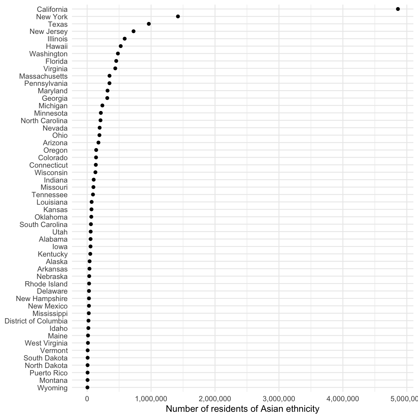
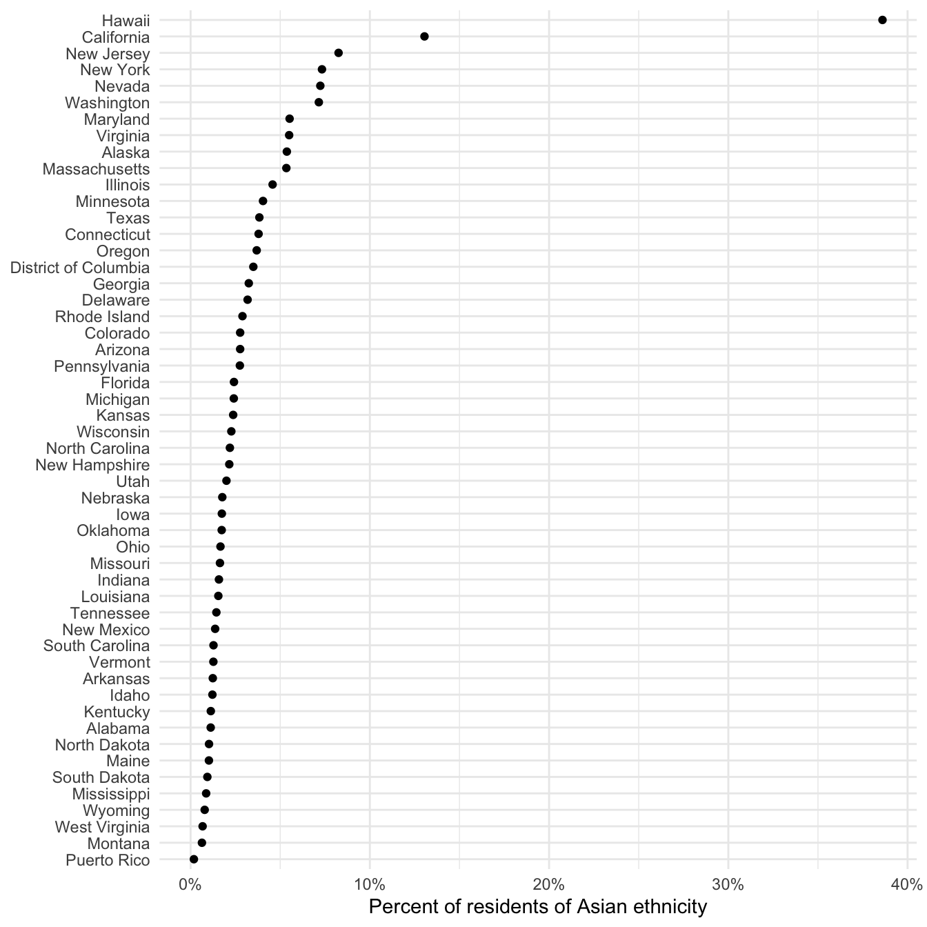
Of course this graph is not entirely useful since it is based on the raw frequency of Asian individuals. California is at the top of the list, but it is also the most populous city. Instead, we could normalize this value as a percentage of the entire state population. To do that, we need to retrieve another variable:
asia_pop <- get_decennial(
  geography = "state",
  variables = c("P008006", "P008001"),
  year = 2010
) %>%
  spread(variable, value) %>%
  mutate(pct_asia = P008006 / P008001)
## Getting data from the 2010 decennial Census
## Using Census Summary File 1
asia_pop
## # A tibble: 52 × 5
##    GEOID NAME                  P008001 P008006 pct_asia
##    <chr> <chr>                   <dbl>   <dbl>    <dbl>
##  1 01    Alabama               4779736   53595   0.0112
##  2 02    Alaska                 710231   38135   0.0537
##  3 04    Arizona               6392017  176695   0.0276
##  4 05    Arkansas              2915918   36102   0.0124
##  5 06    California           37253956 4861007   0.130
##  6 08    Colorado              5029196  139028   0.0276
##  7 09    Connecticut           3574097  135565   0.0379
##  8 10    Delaware               897934   28549   0.0318
##  9 11    District of Columbia   601723   21056   0.0350
## 10 12    Florida              18801310  454821   0.0242
## # … with 42 more rows
## # ℹ Use `print(n = ...)` to see more rows
ggplot(asia_pop, aes(x = reorder(NAME, pct_asia), y = pct_asia)) +
  geom_point() +
  scale_y_continuous(labels = scales::percent) +
  labs(
    x = NULL,
    y = "Percent of residents of Asian ethnicity"
  ) +
  coord_flip()
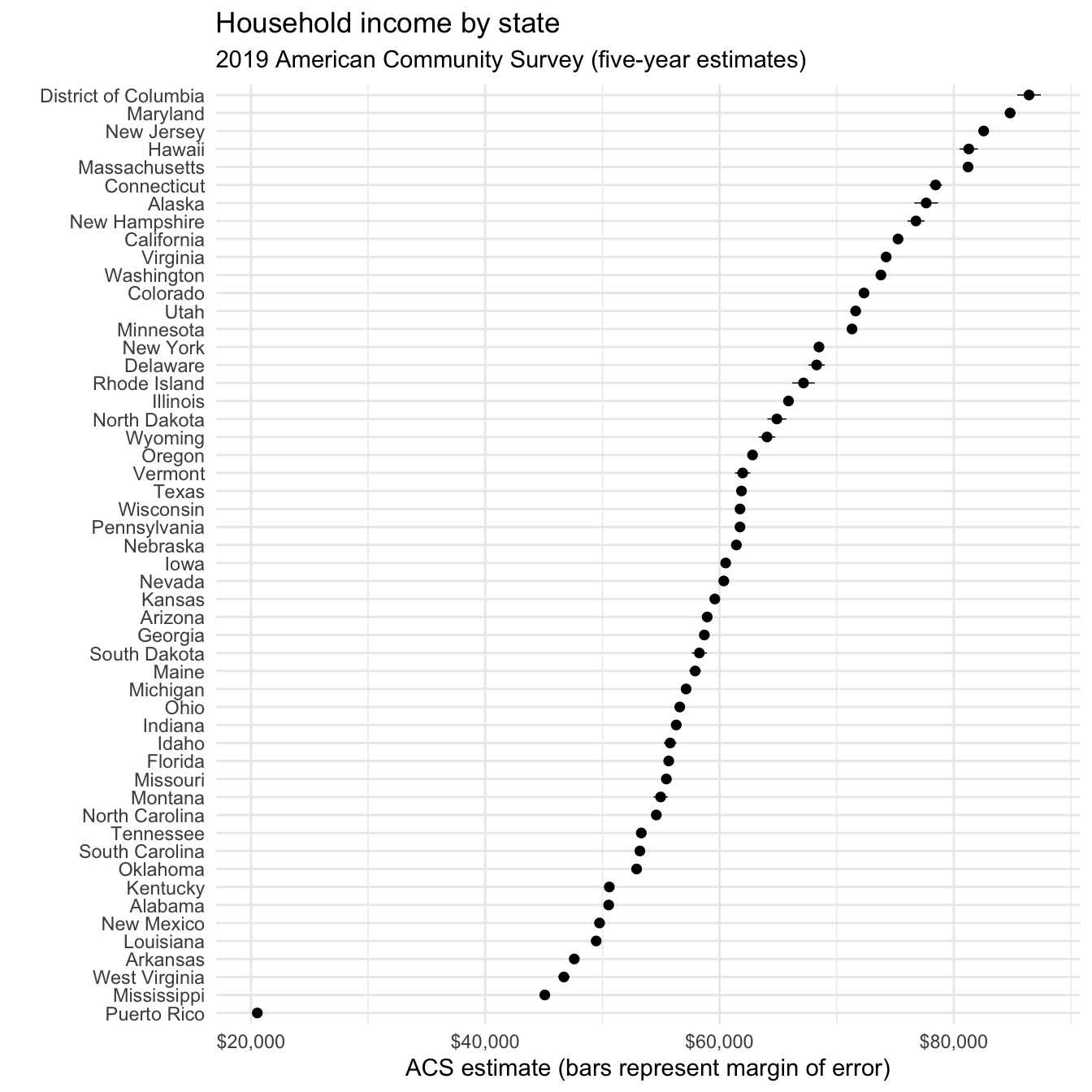
get_acs() retrieves data from the American Community Survey. This survey is administered to a sample of 3 million households on an annual basis, so the data points are estimates characterized by a margin of error. tidycensus returns both the original estimate and margin of error. Let’s get median household income data from the 2014-2019 ACS for each state.
usa_inc <- get_acs(
  geography = "state",
  variables = c(medincome = "B19013_001"),
  year = 2019
)
## Getting data from the 2015-2019 5-year ACS
usa_inc
## # A tibble: 52 × 5
##    GEOID NAME                 variable  estimate   moe
##    <chr> <chr>                <chr>        <dbl> <dbl>
##  1 01    Alabama              medincome    50536   304
##  2 02    Alaska               medincome    77640  1015
##  3 04    Arizona              medincome    58945   266
##  4 05    Arkansas             medincome    47597   328
##  5 06    California           medincome    75235   232
##  6 08    Colorado             medincome    72331   370
##  7 09    Connecticut          medincome    78444   553
##  8 10    Delaware             medincome    68287   696
##  9 11    District of Columbia medincome    86420  1008
## 10 12    Florida              medincome    55660   220
## # … with 42 more rows
## # ℹ Use `print(n = ...)` to see more rows
Now we return both an estimate column for the ACS estimate and moe for the margin of error (defaults to 90% confidence interval).
usa_inc %>%
  ggplot(aes(x = reorder(NAME, estimate), y = estimate)) +
  geom_pointrange(aes(
    ymin = estimate - moe,
    ymax = estimate + moe
  ),
  size = .25
  ) +
  scale_y_continuous(labels = scales::dollar) +
  coord_flip() +
  labs(
    title = "Household income by state",
    subtitle = "2019 American Community Survey (five-year estimates)",
    x = "",
    y = "ACS estimate (bars represent margin of error)"
  )
Search for variables
get_acs() or get_decennial() requires knowing the variable ID, of which there are thousands. load_variables() downloads a list of variable IDs and labels for a given Census or ACS and dataset. You can then use View() to interactively browse through and filter for variables in RStudio.
Drawing maps
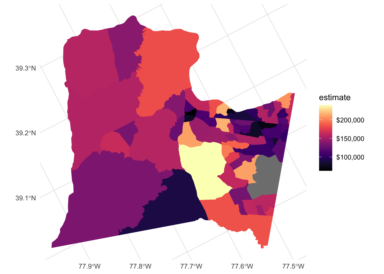
tidycensus also can return simple feature geometry for geographic units along with variables from the decennial Census or ACS, which can then be visualized using geom_sf(). Let’s look at median household income by Census tracts from the 2014-2019 ACS in Loudoun County, Virginia:
loudoun <- get_acs(
  state = "VA",
  county = "Loudoun",
  geography = "tract",
  variables = c(medincome = "B19013_001"),
  year = 2019,
  geometry = TRUE
)
loudoun
## Simple feature collection with 65 features and 5 fields
## Geometry type: MULTIPOLYGON
## Dimension:     XY
## Bounding box:  xmin: -77.9622 ymin: 38.84621 xmax: -77.32828 ymax: 39.32419
## Geodetic CRS:  NAD83
## First 10 features:
##          GEOID                                           NAME  variable
## 1  51107611005 Census Tract 6110.05, Loudoun County, Virginia medincome
## 2  51107611013 Census Tract 6110.13, Loudoun County, Virginia medincome
## 3  51107611010 Census Tract 6110.10, Loudoun County, Virginia medincome
## 4  51107611802 Census Tract 6118.02, Loudoun County, Virginia medincome
## 5  51107610504 Census Tract 6105.04, Loudoun County, Virginia medincome
## 6  51107611300    Census Tract 6113, Loudoun County, Virginia medincome
## 7  51107610702 Census Tract 6107.02, Loudoun County, Virginia medincome
## 8  51107611602 Census Tract 6116.02, Loudoun County, Virginia medincome
## 9  51107611601 Census Tract 6116.01, Loudoun County, Virginia medincome
## 10 51107611014 Census Tract 6110.14, Loudoun County, Virginia medincome
##    estimate   moe                       geometry
## 1    140464 12264 MULTIPOLYGON (((-77.50754 3...
## 2    162390 14937 MULTIPOLYGON (((-77.50032 3...
## 3     68162 21264 MULTIPOLYGON (((-77.48152 3...
## 4    161125 16451 MULTIPOLYGON (((-77.54472 3...
## 5    112351 11625 MULTIPOLYGON (((-77.56114 3...
## 6    115145 15114 MULTIPOLYGON (((-77.39662 3...
## 7    132958  9530 MULTIPOLYGON (((-77.72496 3...
## 8     83356 19510 MULTIPOLYGON (((-77.42181 3...
## 9    102125 16320 MULTIPOLYGON (((-77.43496 3...
## 10   119877 12721 MULTIPOLYGON (((-77.48567 3...
This looks similar to the previous output but because we set geometry = TRUE it is now a simple features data frame with a geometry column defining the geographic feature. We can visualize it using geom_sf() and viridis::scale_*_viridis() to adjust the color palette.
ggplot(data = loudoun) +
  geom_sf(mapping = aes(fill = estimate, color = estimate)) +
  coord_sf(crs = 26911) +
  scale_fill_viridis(
    option = "magma",
    labels = scales::dollar,
    aesthetics = c("fill", "color")
  )
Acknowledgments
- This page is derived in part from “UBC STAT 545A and 547M”, licensed under the CC BY-NC 3.0 Creative Commons License.
- Explanation of APIs drawn from Rochelle Terman’s Collecting Data from the Web
Session Info
sessioninfo::session_info()
## ─ Session info ───────────────────────────────────────────────────────────────
##  setting  value
##  version  R version 4.2.1 (2022-06-23)
##  os       macOS Monterey 12.3
##  system   aarch64, darwin20
##  ui       X11
##  language (EN)
##  collate  en_US.UTF-8
##  ctype    en_US.UTF-8
##  tz       America/New_York
##  date     2022-08-22
##  pandoc   2.18 @ /Applications/RStudio.app/Contents/MacOS/quarto/bin/tools/ (via rmarkdown)
##
## ─ Packages ───────────────────────────────────────────────────────────────────
##  package       * version    date (UTC) lib source
##  assertthat      0.2.1      2019-03-21 [2] CRAN (R 4.2.0)
##  backports       1.4.1      2021-12-13 [2] CRAN (R 4.2.0)
##  base64enc       0.1-3      2015-07-28 [2] CRAN (R 4.2.0)
##  blogdown        1.10       2022-05-10 [2] CRAN (R 4.2.0)
##  bookdown        0.27       2022-06-14 [2] CRAN (R 4.2.0)
##  broom         * 1.0.0      2022-07-01 [2] CRAN (R 4.2.0)
##  bslib           0.4.0      2022-07-16 [2] CRAN (R 4.2.0)
##  cachem          1.0.6      2021-08-19 [2] CRAN (R 4.2.0)
##  cellranger      1.1.0      2016-07-27 [2] CRAN (R 4.2.0)
##  cli             3.3.0      2022-04-25 [2] CRAN (R 4.2.0)
##  colorspace      2.0-3      2022-02-21 [2] CRAN (R 4.2.0)
##  crayon          1.5.1      2022-03-26 [2] CRAN (R 4.2.0)
##  DBI             1.1.3      2022-06-18 [2] CRAN (R 4.2.0)
##  dbplyr          2.2.1      2022-06-27 [2] CRAN (R 4.2.0)
##  digest          0.6.29     2021-12-01 [2] CRAN (R 4.2.0)
##  dplyr         * 1.0.9      2022-04-28 [2] CRAN (R 4.2.0)
##  DT              0.23       2022-05-10 [2] CRAN (R 4.2.0)
##  ellipsis        0.3.2      2021-04-29 [2] CRAN (R 4.2.0)
##  evaluate        0.16       2022-08-09 [1] CRAN (R 4.2.1)
##  fansi           1.0.3      2022-03-24 [2] CRAN (R 4.2.0)
##  fastmap         1.1.0      2021-01-25 [2] CRAN (R 4.2.0)
##  forcats       * 0.5.1      2021-01-27 [2] CRAN (R 4.2.0)
##  fs              1.5.2      2021-12-08 [2] CRAN (R 4.2.0)
##  functional      0.6        2014-07-16 [2] CRAN (R 4.2.0)
##  gargle          1.2.0      2021-07-02 [2] CRAN (R 4.2.0)
##  generics        0.1.3      2022-07-05 [2] CRAN (R 4.2.0)
##  ggplot2       * 3.3.6      2022-05-03 [2] CRAN (R 4.2.0)
##  glue            1.6.2      2022-02-24 [2] CRAN (R 4.2.0)
##  googledrive     2.0.0      2021-07-08 [2] CRAN (R 4.2.0)
##  googlesheets4   1.0.0      2021-07-21 [2] CRAN (R 4.2.0)
##  gridExtra       2.3        2017-09-09 [2] CRAN (R 4.2.0)
##  gtable          0.3.0      2019-03-25 [2] CRAN (R 4.2.0)
##  haven           2.5.0      2022-04-15 [2] CRAN (R 4.2.0)
##  here            1.0.1      2020-12-13 [2] CRAN (R 4.2.0)
##  hms             1.1.1      2021-09-26 [2] CRAN (R 4.2.0)
##  htmltools       0.5.3      2022-07-18 [2] CRAN (R 4.2.0)
##  htmlwidgets     1.5.4      2021-09-08 [2] CRAN (R 4.2.0)
##  httr            1.4.3      2022-05-04 [2] CRAN (R 4.2.0)
##  janeaustenr     0.1.5      2017-06-10 [2] CRAN (R 4.2.0)
##  jquerylib       0.1.4      2021-04-26 [2] CRAN (R 4.2.0)
##  jsonlite        1.8.0      2022-02-22 [2] CRAN (R 4.2.0)
##  knitr           1.39       2022-04-26 [2] CRAN (R 4.2.0)
##  lattice         0.20-45    2021-09-22 [2] CRAN (R 4.2.1)
##  lifecycle       1.0.1      2021-09-24 [2] CRAN (R 4.2.0)
##  lubridate       1.8.0      2021-10-07 [2] CRAN (R 4.2.0)
##  magrittr        2.0.3      2022-03-30 [2] CRAN (R 4.2.0)
##  manifestoR    * 1.5.0      2020-11-29 [2] CRAN (R 4.2.0)
##  Matrix          1.4-1      2022-03-23 [2] CRAN (R 4.2.1)
##  mnormt          2.1.0      2022-06-07 [2] CRAN (R 4.2.0)
##  modelr          0.1.8      2020-05-19 [2] CRAN (R 4.2.0)
##  munsell         0.5.0      2018-06-12 [2] CRAN (R 4.2.0)
##  nlme            3.1-158    2022-06-15 [2] CRAN (R 4.2.0)
##  NLP           * 0.2-1      2020-10-14 [2] CRAN (R 4.2.0)
##  pillar          1.8.0      2022-07-18 [2] CRAN (R 4.2.0)
##  pkgconfig       2.0.3      2019-09-22 [2] CRAN (R 4.2.0)
##  psych           2.2.5      2022-05-10 [2] CRAN (R 4.2.0)
##  purrr         * 0.3.4      2020-04-17 [2] CRAN (R 4.2.0)
##  R6              2.5.1      2021-08-19 [2] CRAN (R 4.2.0)
##  RColorBrewer  * 1.1-3      2022-04-03 [2] CRAN (R 4.2.0)
##  Rcpp            1.0.9      2022-07-08 [2] CRAN (R 4.2.0)
##  readr         * 2.1.2      2022-01-30 [2] CRAN (R 4.2.0)
##  readxl          1.4.0      2022-03-28 [2] CRAN (R 4.2.0)
##  reprex          2.0.1.9000 2022-08-10 [1] Github (tidyverse/reprex@6d3ad07)
##  rlang           1.0.4      2022-07-12 [2] CRAN (R 4.2.0)
##  rmarkdown       2.14       2022-04-25 [2] CRAN (R 4.2.0)
##  rprojroot       2.0.3      2022-04-02 [2] CRAN (R 4.2.0)
##  rstudioapi      0.13       2020-11-12 [2] CRAN (R 4.2.0)
##  rvest           1.0.2      2021-10-16 [2] CRAN (R 4.2.0)
##  sass            0.4.2      2022-07-16 [2] CRAN (R 4.2.0)
##  scales          1.2.0      2022-04-13 [2] CRAN (R 4.2.0)
##  sessioninfo     1.2.2      2021-12-06 [2] CRAN (R 4.2.0)
##  slam            0.1-50     2022-01-08 [2] CRAN (R 4.2.0)
##  SnowballC       0.7.0      2020-04-01 [2] CRAN (R 4.2.0)
##  stringi         1.7.8      2022-07-11 [2] CRAN (R 4.2.0)
##  stringr       * 1.4.0      2019-02-10 [2] CRAN (R 4.2.0)
##  tibble        * 3.1.8      2022-07-22 [2] CRAN (R 4.2.0)
##  tidyr         * 1.2.0      2022-02-01 [2] CRAN (R 4.2.0)
##  tidyselect      1.1.2      2022-02-21 [2] CRAN (R 4.2.0)
##  tidytext      * 0.3.3      2022-05-09 [2] CRAN (R 4.2.0)
##  tidyverse     * 1.3.2      2022-07-18 [2] CRAN (R 4.2.0)
##  tm            * 0.7-8      2020-11-18 [2] CRAN (R 4.2.0)
##  tokenizers      0.2.1      2018-03-29 [2] CRAN (R 4.2.0)
##  tzdb            0.3.0      2022-03-28 [2] CRAN (R 4.2.0)
##  utf8            1.2.2      2021-07-24 [2] CRAN (R 4.2.0)
##  vctrs           0.4.1      2022-04-13 [2] CRAN (R 4.2.0)
##  viridis       * 0.6.2      2021-10-13 [2] CRAN (R 4.2.0)
##  viridisLite   * 0.4.0      2021-04-13 [2] CRAN (R 4.2.0)
##  wbstats       * 1.0.4      2020-12-05 [2] CRAN (R 4.2.0)
##  withr           2.5.0      2022-03-03 [2] CRAN (R 4.2.0)
##  wordcloud     * 2.6        2018-08-24 [2] CRAN (R 4.2.0)
##  xfun            0.31       2022-05-10 [1] CRAN (R 4.2.0)
##  xml2            1.3.3      2021-11-30 [2] CRAN (R 4.2.0)
##  yaml            2.3.5      2022-02-21 [2] CRAN (R 4.2.0)
##  zoo             1.8-10     2022-04-15 [2] CRAN (R 4.2.0)
##
##  [1] /Users/soltoffbc/Library/R/arm64/4.2/library
##  [2] /Library/Frameworks/R.framework/Versions/4.2-arm64/Resources/library
##
## ──────────────────────────────────────────────────────────────────────────────
Alternatively, you can use the web interface to determine specific indicators and their IDs. ↩︎