Topic modeling
library(tidyverse)
library(tidymodels)
library(tidytext)
library(textrecipes)
library(topicmodels)
library(here)
library(rjson)
library(tm)
library(tictoc)
library(appa)

set.seed(1234)
theme_set(theme_minimal())
Typically when we search for information online, there are two primary methods:
- Keywords - use a search engine and type in words that relate to whatever it is we want to find
- Links - use the networked structure of the web to travel from page to page. Linked pages are likely to share similar or related content.
An alternative method would be to search and explore documents via themes. For instance, David Blei proposes searching through the complete history of the New York Times. Broad themes may relate to the individual sections in the paper (foreign policy, national affairs, sports) but there might be specific themes within or across these sections (Chinese foreign policy, the conflict in the Middle East, the U.S.’s relationship with Russia). If the documents are grouped by these themes, we could track the evolution of the NYT’s reporting on these issues over time, or examine how discussion of different themes intersects.
In order to do this, we would need detailed information on the theme of every article. Hand-coding this corpus would be exceedingly time-consuming, not to mention would requiring knowing the thematic structure of the documents before one even begins coding. For the vast majority of corpa, this is not a feasible approach.
Instead, we can use probabilistic topic models, statistical algorithms that analyze words in original text documents to uncover the thematic structure of the both the corpus and individual documents themselves. They do not require any hand coding or labeling of the documents prior to analysis - instead, the algorithms emerge from the analysis of the text.
Latent Dirichlet allocation
LDA assumes that each document in a corpus contains a mix of topics that are found throughout the entire corpus. The topic structure is hidden - we can only observe the documents and words, not the topics themselves. Because the structure is hidden (also known as latent), this method seeks to infer the topic structure given the known words and documents.
Food and animals
Suppose you have the following set of sentences:
- I ate a banana and spinach smoothie for breakfast.
- I like to eat broccoli and bananas.
- Chinchillas and kittens are cute.
- My sister adopted a kitten yesterday.
- Look at this cute hamster munching on a piece of broccoli.
Latent Dirichlet allocation is a way of automatically discovering topics that these sentences contain. For example, given these sentences and asked for 2 topics, LDA might produce something like
Sentences 1 and 2: 100% Topic A
Sentences 3 and 4: 100% Topic B
Sentence 5: 60% Topic A, 40% Topic B
Topic A: 30% broccoli, 15% bananas, 10% breakfast, 10% munching, …
Topic B: 20% chinchillas, 20% kittens, 20% cute, 15% hamster, …
You could infer that topic A is a topic about food, and topic B is a topic about cute animals. But LDA does not explicitly identify topics in this manner. All it can do is tell you the probability that specific words are associated with the topic.
An LDA document structure
LDA represents documents as mixtures of topics that spit out words with certain probabilities. It assumes that documents are produced in the following fashion: when writing each document, you
- Decide on the number of words $N$ the document will have
- Choose a topic mixture for the document (according to a Dirichlet probability distribution over a fixed set of $K$ topics). For example, assuming that we have the two food and cute animal topics above, you might choose the document to consist of 1/3 food and 2/3 cute animals.
- Generate each word in the document by:
- First picking a topic (according to the distribution that you sampled above; for example, you might pick the food topic with 1/3 probability and the cute animals topic with 2/3 probability).
- Then using the topic to generate the word itself (according to the topic’s multinomial distribution). For instance, the food topic might output the word “broccoli” with 30% probability, “bananas” with 15% probability, and so on.
Assuming this generative model for a collection of documents, LDA then tries to backtrack from the documents to find a set of topics that are likely to have generated the collection.
Food and animals
How could we have generated the sentences in the previous example? When generating a document $D$:
- Decide that $D$ will be 1/2 about food and 1/2 about cute animals.
- Pick 5 to be the number of words in $D$.
- Pick the first word to come from the food topic, which then gives you the word “broccoli”.
- Pick the second word to come from the cute animals topic, which gives you “panda”.
- Pick the third word to come from the cute animals topic, giving you “adorable”.
- Pick the fourth word to come from the food topic, giving you “cherries”.
- Pick the fifth word to come from the food topic, giving you “eating”.
So the document generated under the LDA model will be “broccoli panda adorable cherries eating” (remember that LDA uses a bag-of-words model).
LDA with an unknown topic structure
Frequently when using LDA, you don’t actually know the underlying topic structure of the documents. Generally that is why you are using LDA to analyze the text in the first place. LDA is useful in these instances, but we have to perform additional tests and analysis to confirm that the topic structure uncovered by LDA is a good structure.
appa
![]()
appa contains transcripts from every episode of Avatar: The Last Airbender.1
In this example, we want to explore the underlying themes of the television show through the use of topic modeling. First we need to install and load the package.
remotes::install_github("averyrobbins1/appa")
library(appa)
data("appa")

glimpse(appa)
## Rows: 13,385
## Columns: 12
## $ id <int> 1, 2, 3, 4, 5, 6, 7, 8, 9, 10, 11, 12, 13, 14, 15, 1…
## $ book <fct> Water, Water, Water, Water, Water, Water, Water, Wat…
## $ book_num <int> 1, 1, 1, 1, 1, 1, 1, 1, 1, 1, 1, 1, 1, 1, 1, 1, 1, 1…
## $ chapter <fct> "The Boy in the Iceberg", "The Boy in the Iceberg", …
## $ chapter_num <int> 1, 1, 1, 1, 1, 1, 1, 1, 1, 1, 1, 1, 1, 1, 1, 1, 1, 1…
## $ character <chr> "Katara", "Scene Description", "Sokka", "Scene Descr…
## $ full_text <chr> "Water. Earth. Fire. Air. My grandmother used to tel…
## $ character_words <chr> "Water. Earth. Fire. Air. My grandmother used to tel…
## $ scene_description <list> <>, <>, "[Close-up of the boy as he grins confident…
## $ writer <chr> "Michael Dante DiMartino, Bryan Konietzko, Aaron Eha…
## $ director <chr> "Dave Filoni", "Dave Filoni", "Dave Filoni", "Dave F…
## $ imdb_rating <dbl> 8.1, 8.1, 8.1, 8.1, 8.1, 8.1, 8.1, 8.1, 8.1, 8.1, 8.…
Once we import the data, we can prepare it for the estimating the model. Unlike for supervised text classification, we will use recipes to prepare the data, then convert it into a DocumentTermMatrix to fit the LDA model.
tidymodels framework, unsupervised learning is typically implemented as a recipe step as opposed to a model (remember that unlike supervised learning, unsupervised learning approaches have no outcome of interest to predict). textrecipes includes step_lda() which can be used to directly fit an LDA model as part of the recipe. Unfortunately it does not support deeper methods for exploring and interpreting the results of the model like we use below.appa_rec <- recipe(~ id + character_words, data = appa) %>%
step_tokenize(character_words) %>%
step_stopwords(character_words, stopword_source = "smart") %>%
step_ngram(character_words, num_tokens = 5, min_num_tokens = 1) %>%
step_tokenfilter(character_words, max_tokens = 5000) %>%
step_tf(character_words)
recipe()- initialize the recipe using theappadata frame. We only need thecharacter_wordscolumn which contains the text we are modeling. We will also retain theidcolumn for tidying further in the workflow.step_tokenize()- perform the tokenization of the text datastep_stopwords()- remove common stopwords (equivalent toanti_join(stop_words))step_ngram()- calculates the $n$-grams based on the remaining tokens.num_tokensandmin_num_tokensallows us to calculate all possible 1-grams, 2-grams, 3-grams, 4-grams, and 5-grams.step_tokenfilter()- dedensify the data set and keep only the most commonly used tokens. Here we will retain the top 2500 tokens. If we retained all unique tokens in the dataset, the LDA model could take an extremely long time to estimate even for a relatively small number of topics.step_tf()- calculate the term-frequency for each unique token in each document
Now that we created the recipe, we have to prepare it using the appa data set and then convert it into a DocumentTermMatrix. prep() allows us to prepare the recipe, while bake() lets us extract the resulting data frame.
appa_prep <- prep(appa_rec)

appa_df <- bake(appa_prep, new_data = NULL)
appa_df %>%
  slice(1:5)
## # A tibble: 5 × 5,000
##      id tf_cha…¹ tf_ch…² tf_ch…³ tf_ch…⁴ tf_ch…⁵ tf_ch…⁶ tf_ch…⁷ tf_ch…⁸ tf_ch…⁹
##   <int>    <dbl>   <dbl>   <dbl>   <dbl>   <dbl>   <dbl>   <dbl>   <dbl>   <dbl>
## 1     1        0       0       0       0       0       0       0       0       0
## 2     2        0       0       0       0       0       0       0       0       0
## 3     3        0       0       0       0       0       0       0       0       0
## 4     4        0       0       0       0       0       0       0       0       0
## 5     5        0       0       0       0       0       0       0       0       0
## # … with 4,990 more variables: tf_character_words_aang_aang_aang <dbl>,
## #   tf_character_words_aang_aang_aang_aang <dbl>,
## #   tf_character_words_aang_aang_aang_aang_aang <dbl>,
## #   tf_character_words_aang_airbending <dbl>,
## #   tf_character_words_aang_avatar <dbl>, tf_character_words_aang_back <dbl>,
## #   tf_character_words_aang_big <dbl>, tf_character_words_aang_coming <dbl>,
## #   tf_character_words_aang_dad <dbl>, …
## # ℹ Use `colnames()` to see all variable names
The resulting data frame is one row per line of dialogue and one column per token. To convert it to a DocumentTermMatrix, we need to first convert it into a tidytext format (one-row-per-token), remove all rows with a frequency of 0 (that is, the token did not appear in the joke), then convert it to a DTM using cast_dtm().
appa_dtm_prep <- appa_df %>%
  pivot_longer(
    cols = -id,
    names_to = "token",
    values_to = "n"
  ) %>%
  filter(n != 0) %>%
  # clean the token column so it just includes the token
  mutate(
    token = str_remove(string = token, pattern = "tf_character_words_")
  )

# id must be consecutive with no gaps
appa_new_id <- appa_dtm_prep %>%
  distinct(id) %>%
  mutate(new_id = row_number())

appa_dtm <- left_join(x = appa_dtm_prep, y = appa_new_id) %>%
  cast_dtm(document = new_id, term = token, value = n)
## Joining, by = "id"
appa_dtm
## <<DocumentTermMatrix (documents: 8822, terms: 4999)>>
## Non-/sparse entries: 40408/44060770
## Sparsity           : 100%
## Maximal term length: 40
## Weighting          : term frequency (tf)
Selecting $k$
Remember that for LDA, you need to specify in advance the number of topics in the underlying topic structure.
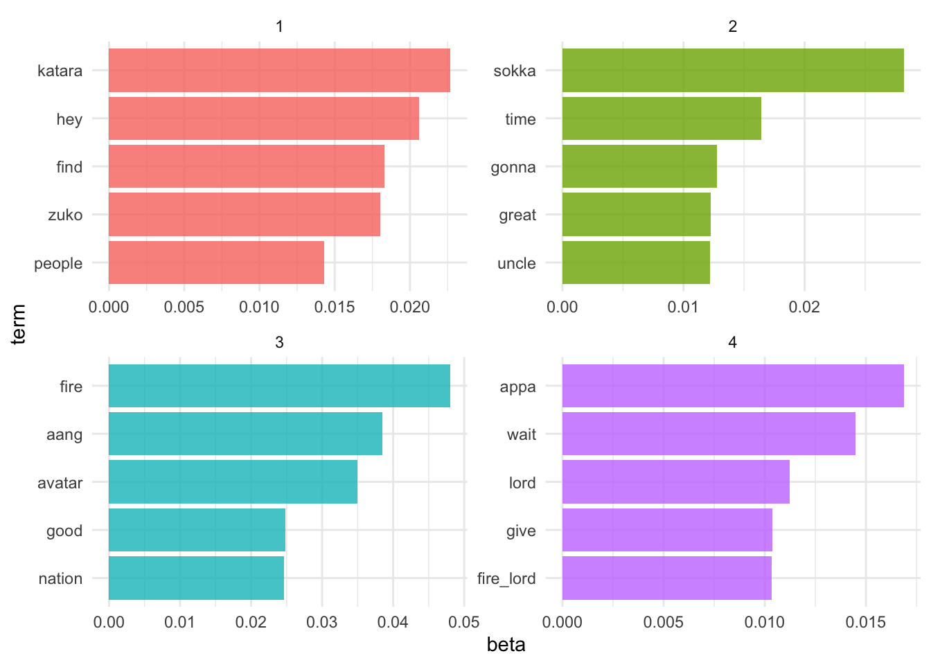
$k=4$
Let’s estimate an LDA model for the transcripts, setting $k=4$.
appa_lda4 <- LDA(appa_dtm, k = 4, control = list(seed = 123))
appa_lda4
## A LDA_VEM topic model with 4 topics.
What do the top terms for each of these topics look like?
appa_lda4_td <- tidy(appa_lda4)

top_terms <- appa_lda4_td %>%
  group_by(topic) %>%
  top_n(5, beta) %>%
  ungroup() %>%
  arrange(topic, -beta)

top_terms %>%
  mutate(
    topic = factor(topic),
    term = reorder_within(term, beta, topic)
  ) %>%
  ggplot(aes(term, beta, fill = topic)) +
  geom_bar(alpha = 0.8, stat = "identity", show.legend = FALSE) +
  scale_x_reordered() +
  facet_wrap(facets = vars(topic), scales = "free", ncol = 2) +
  coord_flip()
$k=12$
What happens if we set $k=12$? How do our results change?
appa_lda12 <- LDA(appa_dtm, k = 12, control = list(seed = 123))
appa_lda12
## A LDA_VEM topic model with 12 topics.
appa_lda12_td <- tidy(appa_lda12)

top_terms <- appa_lda12_td %>%
  group_by(topic) %>%
  top_n(5, beta) %>%
  ungroup() %>%
  arrange(topic, -beta)

top_terms %>%
  mutate(
    topic = factor(topic),
    term = reorder_within(term, beta, topic)
  ) %>%
  ggplot(aes(term, beta, fill = topic)) +
  geom_bar(alpha = 0.8, stat = "identity", show.legend = FALSE) +
  scale_x_reordered() +
  facet_wrap(facets = vars(topic), scales = "free", ncol = 3) +
  coord_flip()
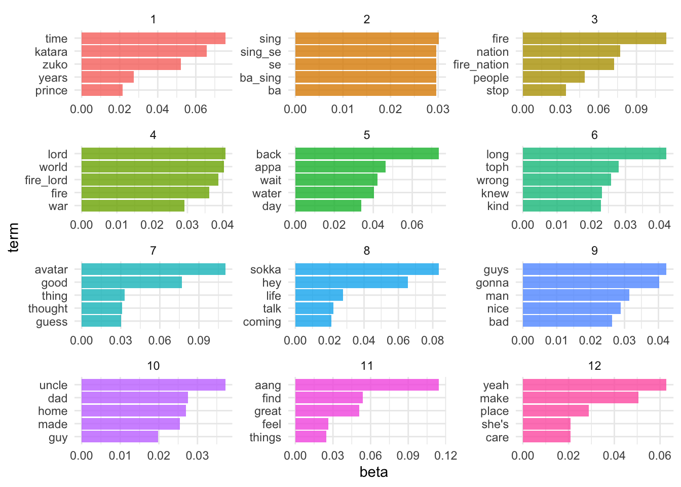
Alas, this is the problem with LDA. Several different values for $k$ may be plausible, but by increasing $k$ we sacrifice clarity. Is there any statistical measure which will help us determine the optimal number of topics?
Perplexity
Well, sort of. Some aspects of LDA are driven by gut-thinking (or perhaps truthiness). However we can have some help. Perplexity is a statistical measure of how well a probability model predicts a sample. As applied to LDA, for a given value of $k$, you estimate the LDA model. Then given the theoretical word distributions represented by the topics, compare that to the actual topic mixtures, or distribution of words in your documents.
topicmodels includes the function perplexity() which calculates this value for a given model.
perplexity(appa_lda12)
## [1] 1373.945
However, the statistic is somewhat meaningless on its own. The benefit of this statistic comes in comparing perplexity across different models with varying $k$s. The model with the lowest perplexity is generally considered the “best”.
Let’s estimate a series of LDA models on the ATLA dataset. Here I make use of purrr and the map() functions to iteratively generate a series of LDA models for the corpus, using a different number of topics in each model.2
n_topics <- c(2, 4, 10, 20, 50, 100)

# cache the models and only estimate if they don't already exist
if (file.exists(here("static", "extras", "appa-lda-compare.Rdata"))) {
  load(file = here("static", "extras", "appa-lda-compare.Rdata"))
} else {
  library(furrr)
  plan(multiprocess)

  tic()
  appa_lda_compare <- n_topics %>%
    future_map(LDA, x = appa_dtm, control = list(seed = 123), .progress = TRUE)
  toc()
  save(appa_dtm, appa_lda_compare, file = here("static", "extras", "appa-lda-compare.Rdata"))
}
tibble(
  k = n_topics,
  perplex = map_dbl(appa_lda_compare, perplexity)
) %>%
  ggplot(aes(k, perplex)) +
  geom_point() +
  geom_line() +
  labs(
    title = "Evaluating LDA topic models",
    subtitle = "Optimal number of topics (smaller is better)",
    x = "Number of topics",
    y = "Perplexity"
  )
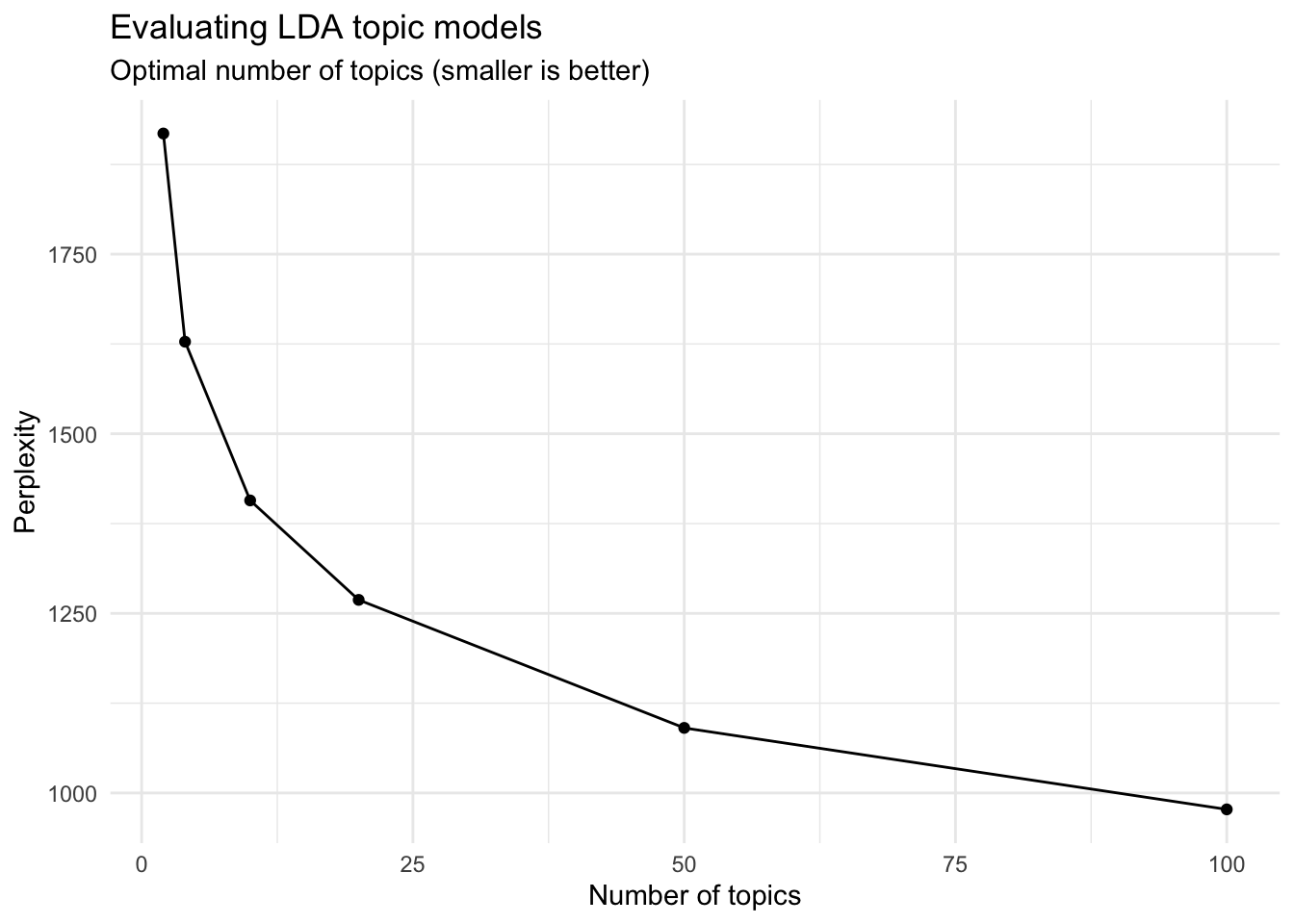
It looks like the 100-topic model has the lowest perplexity score. What kind of topics does this generate? Let’s look just at the first 12 topics produced by the model (ggplot2 has difficulty rendering a graph for 100 separate facets):
appa_lda_td <- tidy(appa_lda_compare[[6]])

top_terms <- appa_lda_td %>%
  group_by(topic) %>%
  top_n(5, beta) %>%
  ungroup() %>%
  arrange(topic, -beta)

top_terms %>%
  filter(topic <= 12) %>%
  mutate(
    topic = factor(topic),
    term = reorder_within(term, beta, topic)
  ) %>%
  ggplot(aes(term, beta, fill = topic)) +
  geom_bar(alpha = 0.8, stat = "identity", show.legend = FALSE) +
  scale_x_reordered() +
  facet_wrap(facets = vars(topic), scales = "free", ncol = 3) +
  coord_flip()
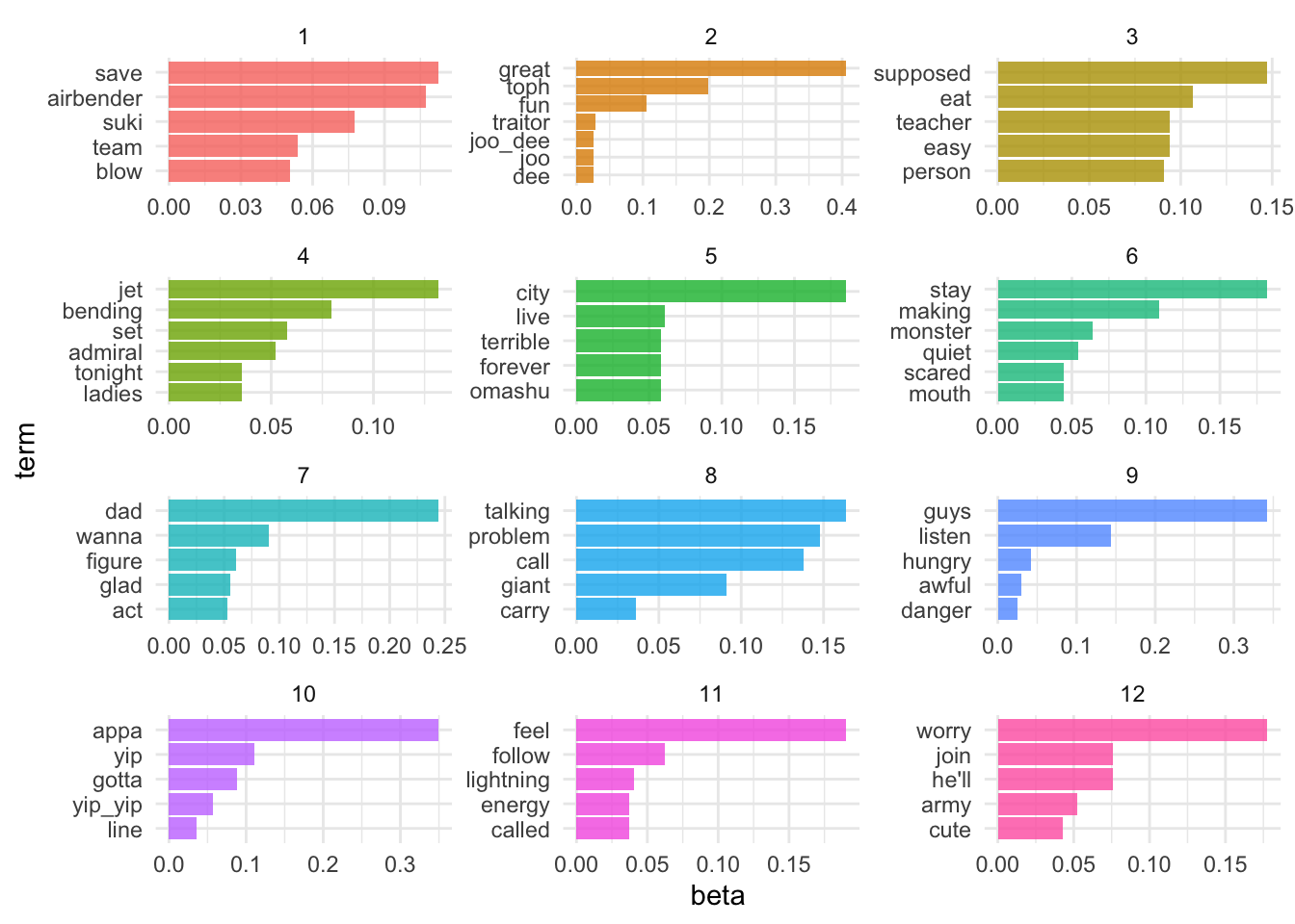
We are getting even more specific topics now. The question becomes how would we present these results and use them in an informative way? Not to mention perplexity was still dropping at $k=100$ - would $k=200$ generate an even lower perplexity score?3
Again, this is where your intuition and domain knowledge as a researcher is important. You can use perplexity as one data point in your decision process, but a lot of the time it helps to simply look at the topics themselves and the highest probability words associated with each one to determine if the structure makes sense. If you have a known topic structure you can compare it to (such as the books example above), this can also be useful.
Interactive exploration of LDA model
The LDAvis allows you to interactively visualize an LDA topic model. The major graphical elements include:
- Default topic circles - $K$ circles, one for each topic, whose areas are set to be proportional to the proportions of the topics across the $N$ total tokens in the corpus.
- Red bars - represent the estimated number of times a given term was generated by a given topic.
- Blue bars - represent the overall frequency of each term in the corpus
- Topic-term circlues - $K \times W$ circles whose areas are set to be proportional to the frequencies with which a given term is estimated to have been generated by the topics.
To install the necessary packages, run the code below:
install.packages("LDAvis")
remotes::install_github("cpsievert/LDAvisData")
Example: This is Jeopardy!
Here we draw an example directly from the LDAvis package to visualize a $K = 100$ topic LDA model of 200,000+ Jeopardy! “answers” and categories. The model is pre-generated and relevant components from the LDA() function are already stored in a list for us. In order to visualize the model, we need to convert this to a JSON file using createJSON() and then pass this object to serVis().
library(LDAvis)

# retrieve LDA model results
data(Jeopardy, package = "LDAvisData")
str(Jeopardy)
## List of 5
##  $ phi           : num [1:100, 1:4393] 9.78e-04 3.51e-06 1.31e-02 4.14e-06 4.31e-06 ...
##   ..- attr(*, "dimnames")=List of 2
##   .. ..$ : chr [1:100] "1" "2" "3" "4" ...
##   .. ..$ : chr [1:4393] "one" "name" "first" "city" ...
##  $ theta         : num [1:19979, 1:100] 0.001111 0.001 0.00125 0.001111 0.000909 ...
##   ..- attr(*, "dimnames")=List of 2
##   .. ..$ : NULL
##   .. ..$ : chr [1:100] "1" "2" "3" "4" ...
##  $ doc.length    : int [1:19979] 8 9 7 8 10 7 5 9 7 13 ...
##  $ vocab         : chr [1:4393] "one" "name" "first" "city" ...
##  $ term.frequency: int [1:4393] 1267 1154 1103 730 715 714 667 659 582 564 ...
# define custom function for approximating distance between topics
library(tsne)
svd_tsne <- function(x) tsne(svd(x)$u)

# convert to JSON file
json <- createJSON(
  phi = Jeopardy$phi,
  theta = Jeopardy$theta,
  doc.length = Jeopardy$doc.length,
  vocab = Jeopardy$vocab,
  term.frequency = Jeopardy$term.frequency,
  mds.method = svd_tsne
)
# view the visualization
serVis(json)
- Check out topic 22 (bodies of water) and 95 (“rhyme time”)
Importing our own LDA model
To convert the output of topicmodels::LDA() to view with LDAvis, use sentopics::as.LDA():
as.LDA() with library(sentopics) (which introduces conflicts with the LDA() function in topicmodels), I use :: notation to access the functions directly.appa_100_viz <- sentopics::as.LDA(appa_lda_compare[[6]], docs = appa_dtm)
sentopics::LDAvis(appa_100_viz, mds.method = svd_tsne)
Acknowledgments
- This page is derived in part from “Tidy Text Mining with R” and licensed under a Creative Commons Attribution-NonCommercial-ShareAlike 3.0 United States License.
- This page is derived in part from “What is a good explanation of Latent Dirichlet Allocation?”
Session Info
sessioninfo::session_info()
## ─ Session info ───────────────────────────────────────────────────────────────
##  setting  value
##  version  R version 4.2.1 (2022-06-23)
##  os       macOS Monterey 12.3
##  system   aarch64, darwin20
##  ui       X11
##  language (EN)
##  collate  en_US.UTF-8
##  ctype    en_US.UTF-8
##  tz       America/New_York
##  date     2022-08-22
##  pandoc   2.18 @ /Applications/RStudio.app/Contents/MacOS/quarto/bin/tools/ (via rmarkdown)
##
## ─ Packages ───────────────────────────────────────────────────────────────────
##  package       * version    date (UTC) lib source
##  appa          * 0.0.0.9000 2022-08-11 [1] Github (averyrobbins1/appa@c7ce69d)
##  assertthat      0.2.1      2019-03-21 [2] CRAN (R 4.2.0)
##  backports       1.4.1      2021-12-13 [2] CRAN (R 4.2.0)
##  blogdown        1.10       2022-05-10 [2] CRAN (R 4.2.0)
##  bookdown        0.27       2022-06-14 [2] CRAN (R 4.2.0)
##  broom         * 1.0.0      2022-07-01 [2] CRAN (R 4.2.0)
##  bslib           0.4.0      2022-07-16 [2] CRAN (R 4.2.0)
##  cachem          1.0.6      2021-08-19 [2] CRAN (R 4.2.0)
##  cellranger      1.1.0      2016-07-27 [2] CRAN (R 4.2.0)
##  class           7.3-20     2022-01-16 [2] CRAN (R 4.2.1)
##  cli             3.3.0      2022-04-25 [2] CRAN (R 4.2.0)
##  codetools       0.2-18     2020-11-04 [2] CRAN (R 4.2.1)
##  colorspace      2.0-3      2022-02-21 [2] CRAN (R 4.2.0)
##  crayon          1.5.1      2022-03-26 [2] CRAN (R 4.2.0)
##  DBI             1.1.3      2022-06-18 [2] CRAN (R 4.2.0)
##  dbplyr          2.2.1      2022-06-27 [2] CRAN (R 4.2.0)
##  dials         * 1.0.0      2022-06-14 [2] CRAN (R 4.2.0)
##  DiceDesign      1.9        2021-02-13 [2] CRAN (R 4.2.0)
##  digest          0.6.29     2021-12-01 [2] CRAN (R 4.2.0)
##  dplyr         * 1.0.9      2022-04-28 [2] CRAN (R 4.2.0)
##  ellipsis        0.3.2      2021-04-29 [2] CRAN (R 4.2.0)
##  evaluate        0.16       2022-08-09 [1] CRAN (R 4.2.1)
##  fansi           1.0.3      2022-03-24 [2] CRAN (R 4.2.0)
##  fastmap         1.1.0      2021-01-25 [2] CRAN (R 4.2.0)
##  forcats       * 0.5.1      2021-01-27 [2] CRAN (R 4.2.0)
##  foreach         1.5.2      2022-02-02 [2] CRAN (R 4.2.0)
##  fs              1.5.2      2021-12-08 [2] CRAN (R 4.2.0)
##  furrr           0.3.0      2022-05-04 [2] CRAN (R 4.2.0)
##  future          1.27.0     2022-07-22 [2] CRAN (R 4.2.0)
##  future.apply    1.9.0      2022-04-25 [2] CRAN (R 4.2.0)
##  gargle          1.2.0      2021-07-02 [2] CRAN (R 4.2.0)
##  generics        0.1.3      2022-07-05 [2] CRAN (R 4.2.0)
##  ggplot2       * 3.3.6      2022-05-03 [2] CRAN (R 4.2.0)
##  globals         0.16.0     2022-08-05 [2] CRAN (R 4.2.0)
##  glue            1.6.2      2022-02-24 [2] CRAN (R 4.2.0)
##  googledrive     2.0.0      2021-07-08 [2] CRAN (R 4.2.0)
##  googlesheets4   1.0.0      2021-07-21 [2] CRAN (R 4.2.0)
##  gower           1.0.0      2022-02-03 [2] CRAN (R 4.2.0)
##  GPfit           1.0-8      2019-02-08 [2] CRAN (R 4.2.0)
##  gtable          0.3.0      2019-03-25 [2] CRAN (R 4.2.0)
##  hardhat         1.2.0      2022-06-30 [2] CRAN (R 4.2.0)
##  haven           2.5.0      2022-04-15 [2] CRAN (R 4.2.0)
##  here          * 1.0.1      2020-12-13 [2] CRAN (R 4.2.0)
##  hms             1.1.1      2021-09-26 [2] CRAN (R 4.2.0)
##  htmltools       0.5.3      2022-07-18 [2] CRAN (R 4.2.0)
##  httr            1.4.3      2022-05-04 [2] CRAN (R 4.2.0)
##  infer         * 1.0.2      2022-06-10 [2] CRAN (R 4.2.0)
##  ipred           0.9-13     2022-06-02 [2] CRAN (R 4.2.0)
##  iterators       1.0.14     2022-02-05 [2] CRAN (R 4.2.0)
##  janeaustenr     0.1.5      2017-06-10 [2] CRAN (R 4.2.0)
##  jquerylib       0.1.4      2021-04-26 [2] CRAN (R 4.2.0)
##  jsonlite        1.8.0      2022-02-22 [2] CRAN (R 4.2.0)
##  knitr           1.39       2022-04-26 [2] CRAN (R 4.2.0)
##  lattice         0.20-45    2021-09-22 [2] CRAN (R 4.2.1)
##  lava            1.6.10     2021-09-02 [2] CRAN (R 4.2.0)
##  lhs             1.1.5      2022-03-22 [2] CRAN (R 4.2.0)
##  lifecycle       1.0.1      2021-09-24 [2] CRAN (R 4.2.0)
##  listenv         0.8.0      2019-12-05 [2] CRAN (R 4.2.0)
##  lubridate       1.8.0      2021-10-07 [2] CRAN (R 4.2.0)
##  magrittr        2.0.3      2022-03-30 [2] CRAN (R 4.2.0)
##  MASS            7.3-58.1   2022-08-03 [2] CRAN (R 4.2.0)
##  Matrix          1.4-1      2022-03-23 [2] CRAN (R 4.2.1)
##  modeldata     * 1.0.0      2022-07-01 [2] CRAN (R 4.2.0)
##  modelr          0.1.8      2020-05-19 [2] CRAN (R 4.2.0)
##  modeltools      0.2-23     2020-03-05 [2] CRAN (R 4.2.0)
##  munsell         0.5.0      2018-06-12 [2] CRAN (R 4.2.0)
##  NLP           * 0.2-1      2020-10-14 [2] CRAN (R 4.2.0)
##  nnet            7.3-17     2022-01-16 [2] CRAN (R 4.2.1)
##  parallelly      1.32.1     2022-07-21 [2] CRAN (R 4.2.0)
##  parsnip       * 1.0.0      2022-06-16 [2] CRAN (R 4.2.0)
##  pillar          1.8.0      2022-07-18 [2] CRAN (R 4.2.0)
##  pkgconfig       2.0.3      2019-09-22 [2] CRAN (R 4.2.0)
##  prodlim         2019.11.13 2019-11-17 [2] CRAN (R 4.2.0)
##  purrr         * 0.3.4      2020-04-17 [2] CRAN (R 4.2.0)
##  R6              2.5.1      2021-08-19 [2] CRAN (R 4.2.0)
##  Rcpp            1.0.9      2022-07-08 [2] CRAN (R 4.2.0)
##  readr         * 2.1.2      2022-01-30 [2] CRAN (R 4.2.0)
##  readxl          1.4.0      2022-03-28 [2] CRAN (R 4.2.0)
##  recipes       * 1.0.1      2022-07-07 [2] CRAN (R 4.2.0)
##  reprex          2.0.1.9000 2022-08-10 [1] Github (tidyverse/reprex@6d3ad07)
##  rjson         * 0.2.21     2022-01-09 [2] CRAN (R 4.2.0)
##  rlang           1.0.4      2022-07-12 [2] CRAN (R 4.2.0)
##  rmarkdown       2.14       2022-04-25 [2] CRAN (R 4.2.0)
##  rpart           4.1.16     2022-01-24 [2] CRAN (R 4.2.1)
##  rprojroot       2.0.3      2022-04-02 [2] CRAN (R 4.2.0)
##  rsample       * 1.1.0      2022-08-08 [2] CRAN (R 4.2.1)
##  rstudioapi      0.13       2020-11-12 [2] CRAN (R 4.2.0)
##  rvest           1.0.2      2021-10-16 [2] CRAN (R 4.2.0)
##  sass            0.4.2      2022-07-16 [2] CRAN (R 4.2.0)
##  scales        * 1.2.0      2022-04-13 [2] CRAN (R 4.2.0)
##  sessioninfo     1.2.2      2021-12-06 [2] CRAN (R 4.2.0)
##  slam            0.1-50     2022-01-08 [2] CRAN (R 4.2.0)
##  SnowballC       0.7.0      2020-04-01 [2] CRAN (R 4.2.0)
##  stringi         1.7.8      2022-07-11 [2] CRAN (R 4.2.0)
##  stringr       * 1.4.0      2019-02-10 [2] CRAN (R 4.2.0)
##  survival        3.3-1      2022-03-03 [2] CRAN (R 4.2.1)
##  textrecipes   * 1.0.0      2022-07-02 [2] CRAN (R 4.2.0)
##  tibble        * 3.1.8      2022-07-22 [2] CRAN (R 4.2.0)
##  tictoc        * 1.0.1      2021-04-19 [2] CRAN (R 4.2.0)
##  tidymodels    * 1.0.0      2022-07-13 [2] CRAN (R 4.2.0)
##  tidyr         * 1.2.0      2022-02-01 [2] CRAN (R 4.2.0)
##  tidyselect      1.1.2      2022-02-21 [2] CRAN (R 4.2.0)
##  tidytext      * 0.3.3      2022-05-09 [2] CRAN (R 4.2.0)
##  tidyverse     * 1.3.2      2022-07-18 [2] CRAN (R 4.2.0)
##  timeDate        4021.104   2022-07-19 [2] CRAN (R 4.2.0)
##  tm            * 0.7-8      2020-11-18 [2] CRAN (R 4.2.0)
##  tokenizers      0.2.1      2018-03-29 [2] CRAN (R 4.2.0)
##  topicmodels   * 0.2-12     2021-01-29 [2] CRAN (R 4.2.0)
##  tune          * 1.0.0      2022-07-07 [2] CRAN (R 4.2.0)
##  tzdb            0.3.0      2022-03-28 [2] CRAN (R 4.2.0)
##  utf8            1.2.2      2021-07-24 [2] CRAN (R 4.2.0)
##  vctrs           0.4.1      2022-04-13 [2] CRAN (R 4.2.0)
##  withr           2.5.0      2022-03-03 [2] CRAN (R 4.2.0)
##  workflows     * 1.0.0      2022-07-05 [2] CRAN (R 4.2.0)
##  workflowsets  * 1.0.0      2022-07-12 [2] CRAN (R 4.2.0)
##  xfun            0.31       2022-05-10 [1] CRAN (R 4.2.0)
##  xml2            1.3.3      2021-11-30 [2] CRAN (R 4.2.0)
##  yaml            2.3.5      2022-02-21 [2] CRAN (R 4.2.0)
##  yardstick     * 1.0.0      2022-06-06 [2] CRAN (R 4.2.0)
##
##  [1] /Users/soltoffbc/Library/R/arm64/4.2/library
##  [2] /Library/Frameworks/R.framework/Versions/4.2-arm64/Resources/library
##
## ──────────────────────────────────────────────────────────────────────────────
Not that nonsense M. Night Shyamalan movie. Or that other Avatar movie. ↩︎
Note that LDA can quickly become CPU and memory intensive as you scale up the size of the corpus and number of topics. Replicating this analysis on your computer may take a long time (i.e. minutes or even hours). It is very possible you may not be able to replicate this analysis on your machine. If so, you need to reduce the amount of text, the number of models, or offload the analysis to a high-performance computing cluster. ↩︎
I tried to estimate this model, but my computer was taking too long. ↩︎