Supervised classification with text data
library(tidyverse)
library(tidymodels)
library(tidytext)

set.seed(1234)
theme_set(theme_minimal())
A common task in social science involves hand-labeling sets of documents for specific variables (e.g. manual coding). In previous years, this required hiring a set of research assistants and training them to read and evaluate text by hand. It was expensive, prone to error, required extensive data quality checks, and was infeasible if you had an extremely large corpus of text that required classification.
Alternatively, we can now use machine learning models to classify text into specific sets of categories. This is known as supervised learning. The basic process is:
- Hand-code a small set of documents (say $N = 1,000$) for whatever variable(s) you care about
- Train a machine learning model on the hand-coded data, using the variable as the outcome of interest and the text features of the documents as the predictors
- Evaluate the effectiveness of the machine learning model via cross-validation
- Once you have trained a model with sufficient predictive accuracy, apply the model to the remaining set of documents that have never been hand-coded (say $N = 1,000,000$)
Sample set of documents: USCongress
# get USCongress data
data(USCongress, package = "rcis")

# topic labels
major_topics <- tibble(
  major = c(1:10, 12:21, 99),
  label = c(
    "Macroeconomics", "Civil rights, minority issues, civil liberties",
    "Health", "Agriculture", "Labor and employment", "Education", "Environment",
    "Energy", "Immigration", "Transportation", "Law, crime, family issues",
    "Social welfare", "Community development and housing issues",
    "Banking, finance, and domestic commerce", "Defense",
    "Space, technology, and communications", "Foreign trade",
    "International affairs and foreign aid", "Government operations",
    "Public lands and water management", "Other, miscellaneous"
  )
)

(congress <- as_tibble(USCongress) %>%
  mutate(text = as.character(text)) %>%
  left_join(major_topics))
## Joining, by = "major"
## # A tibble: 4,449 × 7
##       ID  cong billnum h_or_sen major text                                 label
##    <dbl> <dbl>   <dbl> <chr>    <dbl> <chr>                                <chr>
##  1     1   107    4499 HR          18 To suspend temporarily the duty on … Fore…
##  2     2   107    4500 HR          18 To suspend temporarily the duty on … Fore…
##  3     3   107    4501 HR          18 To suspend temporarily the duty on … Fore…
##  4     4   107    4502 HR          18 To reduce temporarily the duty on P… Fore…
##  5     5   107    4503 HR           5 To amend the Immigration and Nation… Labo…
##  6     6   107    4504 HR          21 To amend title 38, United States Co… Publ…
##  7     7   107    4505 HR          15 To repeal subtitle B of title III o… Bank…
##  8     8   107    4506 HR          18 To suspend temporarily the duty on … Fore…
##  9     9   107    4507 HR          18 To suspend temporarily the duty on … Fore…
## 10    10   107    4508 HR          18 To suspend temporarily the duty on … Fore…
## # … with 4,439 more rows
## # ℹ Use `print(n = ...)` to see more rows
USCongress contains a sample of hand-labeled bills from the United States Congress. For each bill we have a text description of the bill’s purpose (e.g. “To amend the Immigration and Nationality Act in regard to Caribbean-born immigrants.”) as well as the bill’s major policy topic code corresponding to the subject of the bill. There are 20 major policy topics according to this coding scheme (e.g. Macroeconomics, Civil Rights, Health). These topic codes have been labeled by hand. The current dataset only contains a sample of bills from the 107th Congress (2001-03). If we wanted to obtain policy topic codes for all bills introduced over a longer period, we would have to manually code tens of thousands if not millions of bill descriptions. Clearly a task outside of our capabilities.
Instead, we can build a machine learning model which predicts the major topic code of a bill given its text description. These notes outline a potential tidymodels/tidytext workflow for such an approach.
Split the data set
First we need to convert major to a factor variable based on the levels defined in label. Then we can split the data into training and testing datasets using initial_split() from rsample.
set.seed(123)

congress <- congress %>%
  mutate(major = factor(x = major, levels = major, labels = label))

congress_split <- initial_split(data = congress, strata = major, prop = .8)
congress_split
## <Training/Testing/Total>
## <3558/891/4449>
congress_train <- training(congress_split)
congress_test <- testing(congress_split)
Preprocessing the data frame
Next we need to preprocess the data in preparation for modeling. Currently we have text data, and we need to construct numeric, quantitative features for machine learning based on that text. As before, we can use recipes to construct the set of preprocessing steps we want to perform. This time, we only use the text column for the model.
congress_rec <- recipe(major ~ text, data = congress_train)
Now we add steps to process the text of the legislation summaries. We use textrecipes to handle the text variable. First we tokenize the text to words with step_tokenize(). By default this uses tokenizers::tokenize_words(). Next we remove stop words with step_stopwords(); the default choice is the Snowball stop word list, but custom lists can be provided too. Before we calculate tf-idf we use step_tokenfilter() to only keep the 500 most frequent tokens, to avoid creating too many variables in our first model. To finish, we use step_tfidf() to compute tf-idf.
library(textrecipes)

congress_rec <- congress_rec %>%
  step_tokenize(text) %>%
  step_stopwords(text) %>%
  step_tokenfilter(text, max_tokens = 500) %>%
  step_tfidf(text)
Train a model
Using our existing workflow() approach to fitting a model, we can establish a workflow using a relatively straightforward type of classification model: naive Bayes. Naive Bayes is particularly useful as it can handle a large number of features.
library(discrim)
##
## Attaching package: 'discrim'
## The following object is masked from 'package:dials':
##
##     smoothness
nb_spec <- naive_Bayes() %>%
  set_mode("classification") %>%
  set_engine("naivebayes")

nb_spec
## Naive Bayes Model Specification (classification)
##
## Computational engine: naivebayes
nb_wf <- workflow() %>%
  add_recipe(congress_rec) %>%
  add_model(nb_spec)
nb_wf
## ══ Workflow ════════════════════════════════════════════════════════════════════
## Preprocessor: Recipe
## Model: naive_Bayes()
##
## ── Preprocessor ────────────────────────────────────────────────────────────────
## 4 Recipe Steps
##
## • step_tokenize()
## • step_stopwords()
## • step_tokenfilter()
## • step_tfidf()
##
## ── Model ───────────────────────────────────────────────────────────────────────
## Naive Bayes Model Specification (classification)
##
## Computational engine: naivebayes
nb_wf %>%
  fit(data = congress_train)
## ══ Workflow [trained] ══════════════════════════════════════════════════════════
## Preprocessor: Recipe
## Model: naive_Bayes()
##
## ── Preprocessor ────────────────────────────────────────────────────────────────
## 4 Recipe Steps
##
## • step_tokenize()
## • step_stopwords()
## • step_tokenfilter()
## • step_tfidf()
##
## ── Model ───────────────────────────────────────────────────────────────────────
##
## ================================== Naive Bayes ==================================
##
##  Call:
## naive_bayes.default(x = maybe_data_frame(x), y = y, usekernel = TRUE)
##
## ---------------------------------------------------------------------------------
##
## Laplace smoothing: 0
##
## ---------------------------------------------------------------------------------
##
##  A priori probabilities:
##
##                                  Foreign trade
##                                    0.089938168
##                           Labor and employment
##                                    0.059584036
##              Public lands and water management
##                                    0.105115233
##        Banking, finance, and domestic commerce
##                                    0.063518831
##                                        Defense
##                                    0.047498595
##                      Law, crime, family issues
##                                    0.065767285
## Civil rights, minority issues, civil liberties
##                                    0.017987634
##                                         Health
##                                    0.138279933
##          International affairs and foreign aid
##                                    0.026700393
##                          Government operations
##                                    0.086003373
##                           Other, miscellaneous
##                                    0.007588533
##                                 Transportation
##                                    0.039066892
##                                      Education
##                                    0.052276560
##          Space, technology, and communications
##                                    0.019673974
##                                    Environment
##                                    0.042158516
##                                 Macroeconomics
##                                    0.037380551
##                                 Social welfare
##                                    0.020798201
##                                         Energy
##                                    0.033164699
##
## ...
## and 1715 more lines.
Evaluation
As we have already seen, we should not use the test set to compare models or different parameters. Instead, we can use cross-validation to evaluate our model.
Here, let’s reformulate this to use naive Bayes classification with 10-fold cross-validation sets.
set.seed(123)

congress_folds <- vfold_cv(data = congress_train, strata = major)
congress_folds
## #  10-fold cross-validation using stratification
## # A tibble: 10 × 2
##    splits             id
##    <list>             <chr>
##  1 <split [3201/357]> Fold01
##  2 <split [3201/357]> Fold02
##  3 <split [3201/357]> Fold03
##  4 <split [3201/357]> Fold04
##  5 <split [3203/355]> Fold05
##  6 <split [3203/355]> Fold06
##  7 <split [3203/355]> Fold07
##  8 <split [3203/355]> Fold08
##  9 <split [3203/355]> Fold09
## 10 <split [3203/355]> Fold10
nb_cv <- nb_wf %>%
  fit_resamples(
    congress_folds,
    control = control_resamples(save_pred = TRUE)
  )
We can extract relevant information using collect_metrics() and collect_predictions().
nb_cv_metrics <- collect_metrics(nb_cv)
nb_cv_predictions <- collect_predictions(nb_cv)

nb_cv_metrics
## # A tibble: 2 × 6
##   .metric  .estimator  mean     n std_err .config
##   <chr>    <chr>      <dbl> <int>   <dbl> <chr>
## 1 accuracy multiclass 0.139    10 0.00491 Preprocessor1_Model1
## 2 roc_auc  hand_till  0.538    10 0.00391 Preprocessor1_Model1
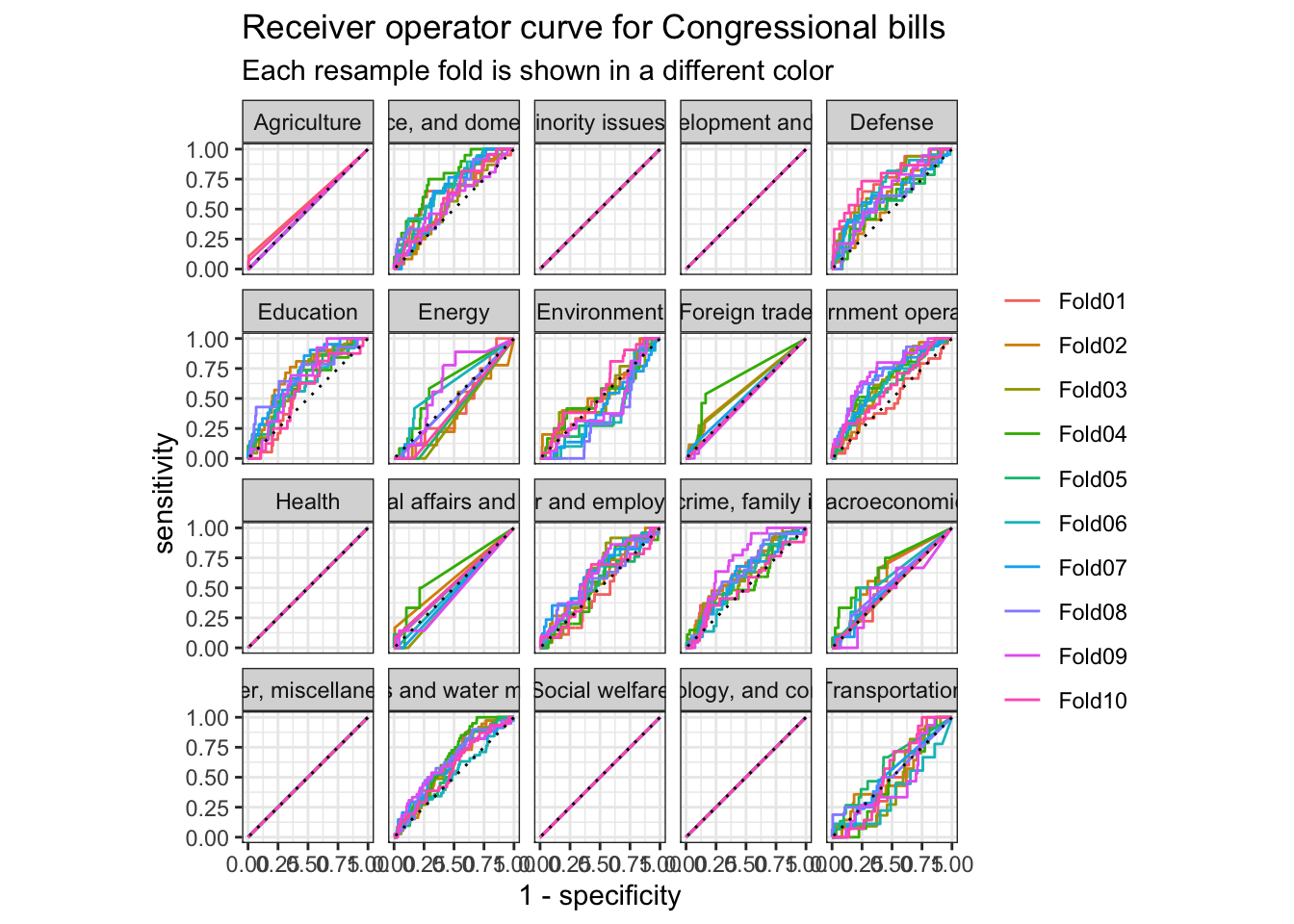
The default performance parameters for multiclass classification are accuracy and ROC AUC (area under the receiver operator curve). The accuracy is the percentage of accurate predictions. For both metrics, values closer to 1 are better. These results suggest the naive Bayes model is performing quite poorly.
The receiver operator curve is a plot that shows the sensitivity at different thresholds. It demonstrates how well a classification model can distinguish between classes.
nb_cv_predictions %>%
  group_by(id) %>%
  roc_curve(truth = major, c(starts_with(".pred"), -.pred_class)) %>%
  autoplot() +
  labs(
    color = NULL,
    title = "Receiver operator curve for Congressional bills",
    subtitle = "Each resample fold is shown in a different color"
  )
Another way to evaluate our model is to evaluate the confusion matrix. A confusion matrix visualizes a model’s false positives and false negatives for each class. Because we implemented 10-fold cross-validation, we actually have 10 confusion matricies. conf_mat_resampled() averages the results from each validation fold to generate the summarized confusion matrix.
conf_mat_resampled(x = nb_cv, tidy = FALSE) %>%
  autoplot(type = "heatmap") +
  scale_y_discrete(labels = function(x) str_wrap(x, 20)) +
  scale_x_discrete(labels = function(x) str_wrap(x, 20))
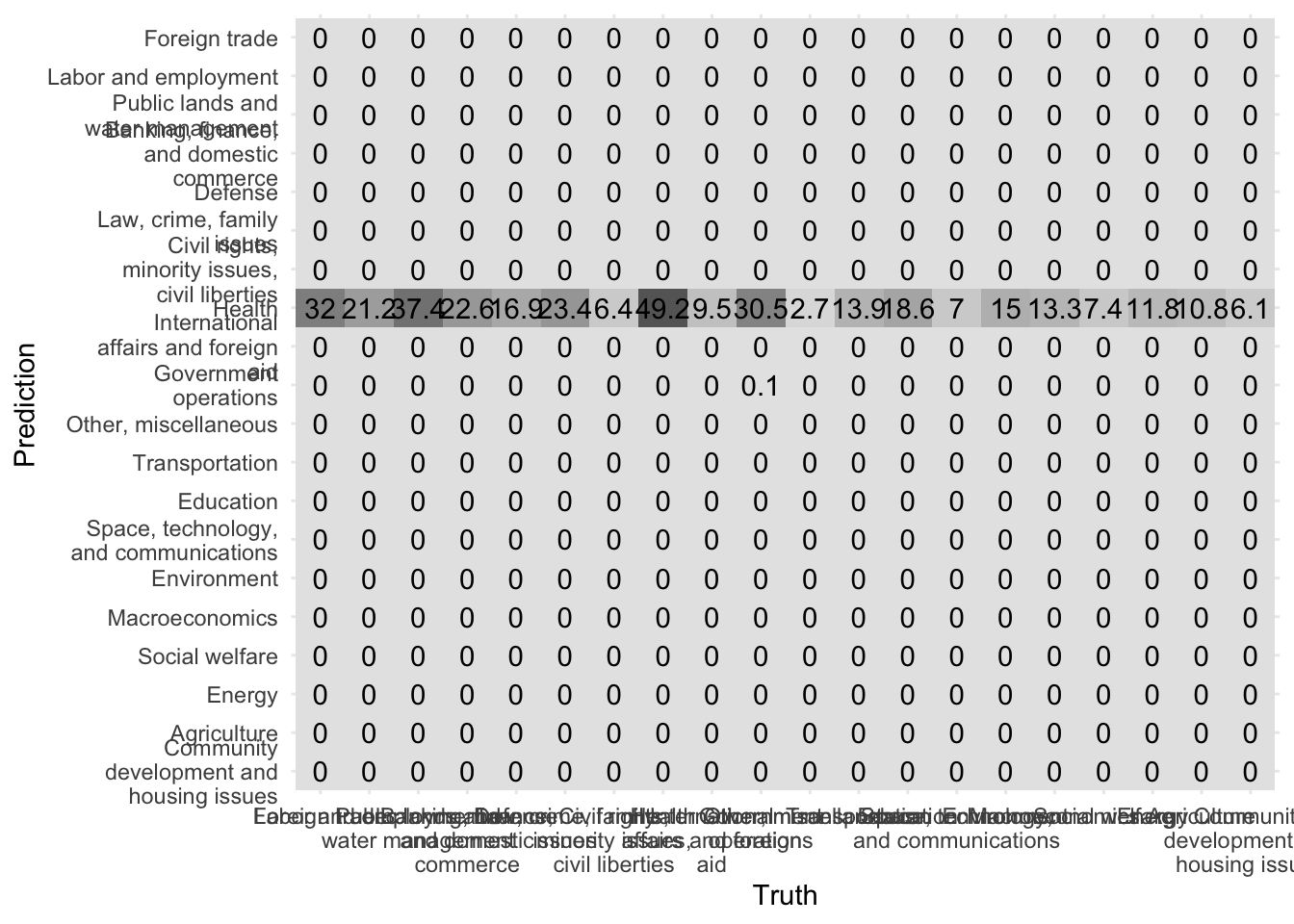
Ideally all observations would fall on the diagonal. However here we can see that all predictions all under “Health” no matter what the true category.
Compare to the null model
We can assess this model by comparing its performance to a “null model”, or a baseline model. This baseline is a simple, non-informative model that always predicts the largest class for classification. In the absence of any information about the individual observations, this is the best strategy we can follow to generate predictions.
null_classification <- null_model() %>%
  set_engine("parsnip") %>%
  set_mode("classification")

null_cv <- workflow() %>%
  add_recipe(congress_rec) %>%
  add_model(null_classification) %>%
  fit_resamples(
    congress_folds
  )

null_cv %>%
  collect_metrics()
## # A tibble: 2 × 6
##   .metric  .estimator  mean     n std_err .config
##   <chr>    <chr>      <dbl> <int>   <dbl> <chr>
## 1 accuracy multiclass 0.138    10 0.00492 Preprocessor1_Model1
## 2 roc_auc  hand_till  0.5      10 0       Preprocessor1_Model1
Notice the accuracy is the same as for the naive Bayes model. This is because naive Bayes still leads to every observation predicted as “Health”, which is the exact same result as the null model. Clearly we need a better modeling strategy.
Concerns regarding multiclass classification
Remember that each bill could fall under one of 20 major policy topics. Compared to binary classification, this is a much harder challenge. For one, the classes are imbalanced. That is, there are far more healthcare related bills than other areas.
ggplot(data = congress, mapping = aes(x = fct_infreq(major) %>% fct_rev())) +
  geom_bar() +
  coord_flip() +
  labs(
    title = "Distribution of legislation",
    subtitle = "By major policy topic",
    x = NULL,
    y = "Number of bills"
  )
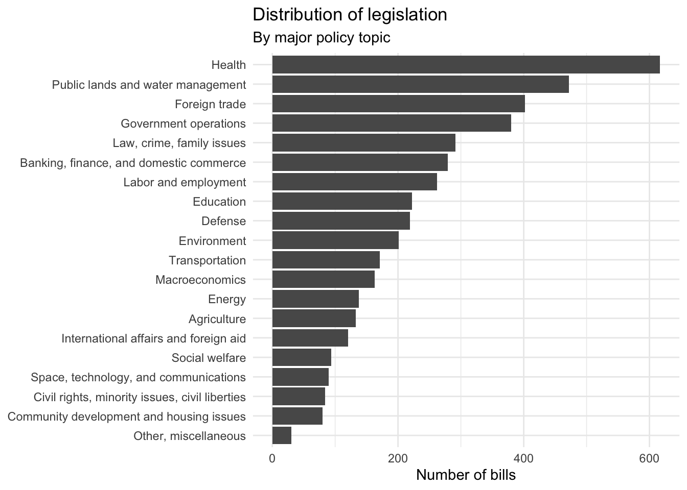
Many machine learning algorithms (such as naive Bayes) do not handle imbalanced data well, while other algorithms may not even be capable of performing multiclass classification.
There are many different ways to deal with imbalanced data. Here we will take a simple approach, downsampling, where observations from the majority classes are removed during training to achieve a balanced class distribution. We rely on the themis package for recipes which includes the step_downsample() function to perform downsampling.
library(themis)

# build on existing recipe
congress_rec <- congress_rec %>%
  step_downsample(major)
congress_rec
## Recipe
##
## Inputs:
##
##       role #variables
##    outcome          1
##  predictor          1
##
## Operations:
##
## Tokenization for text
## Stop word removal for text
## Text filtering for text
## Term frequency-inverse document frequency with text
## Down-sampling based on major
Let’s also switch to an alternative modeling approach which handles multiclass problems better, decision trees.
tree_spec <- decision_tree() %>%
  set_mode("classification") %>%
  set_engine("C5.0")

tree_spec
## Decision Tree Model Specification (classification)
##
## Computational engine: C5.0
tree_wf <- workflow() %>%
  add_recipe(congress_rec) %>%
  add_model(tree_spec)

tree_wf
## ══ Workflow ════════════════════════════════════════════════════════════════════
## Preprocessor: Recipe
## Model: decision_tree()
##
## ── Preprocessor ────────────────────────────────────────────────────────────────
## 5 Recipe Steps
##
## • step_tokenize()
## • step_stopwords()
## • step_tokenfilter()
## • step_tfidf()
## • step_downsample()
##
## ── Model ───────────────────────────────────────────────────────────────────────
## Decision Tree Model Specification (classification)
##
## Computational engine: C5.0
set.seed(123)

tree_cv <- fit_resamples(
  tree_wf,
  congress_folds,
  control = control_resamples(save_pred = TRUE)
)
tree_cv
## # Resampling results
## # 10-fold cross-validation using stratification
## # A tibble: 10 × 5
##    splits             id     .metrics         .notes           .predictions
##    <list>             <chr>  <list>           <list>           <list>
##  1 <split [3201/357]> Fold01 <tibble [2 × 4]> <tibble [0 × 3]> <tibble>
##  2 <split [3201/357]> Fold02 <tibble [2 × 4]> <tibble [0 × 3]> <tibble>
##  3 <split [3201/357]> Fold03 <tibble [2 × 4]> <tibble [0 × 3]> <tibble>
##  4 <split [3201/357]> Fold04 <tibble [2 × 4]> <tibble [0 × 3]> <tibble>
##  5 <split [3203/355]> Fold05 <tibble [2 × 4]> <tibble [0 × 3]> <tibble>
##  6 <split [3203/355]> Fold06 <tibble [2 × 4]> <tibble [0 × 3]> <tibble>
##  7 <split [3203/355]> Fold07 <tibble [2 × 4]> <tibble [0 × 3]> <tibble>
##  8 <split [3203/355]> Fold08 <tibble [2 × 4]> <tibble [0 × 3]> <tibble>
##  9 <split [3203/355]> Fold09 <tibble [2 × 4]> <tibble [0 × 3]> <tibble>
## 10 <split [3203/355]> Fold10 <tibble [2 × 4]> <tibble [0 × 3]> <tibble>
tree_cv_metrics <- collect_metrics(tree_cv)
tree_cv_predictions <- collect_predictions(tree_cv)

tree_cv_metrics
## # A tibble: 2 × 6
##   .metric  .estimator  mean     n std_err .config
##   <chr>    <chr>      <dbl> <int>   <dbl> <chr>
## 1 accuracy multiclass 0.430    10 0.0124  Preprocessor1_Model1
## 2 roc_auc  hand_till  0.760    10 0.00761 Preprocessor1_Model1
While still low, the accuracy has risen substantially compared to the naive Bayes model. This is typical for multiclass models since the classification task is harder than for binary classification - rather than having one right answer and one wrong answer, there is one right answer and nineteen wrong answers.
conf_mat_resampled(x = tree_cv, tidy = FALSE) %>%
  autoplot(type = "heatmap") +
  scale_y_discrete(labels = function(x) str_wrap(x, 20)) +
  scale_x_discrete(labels = function(x) str_wrap(x, 20))
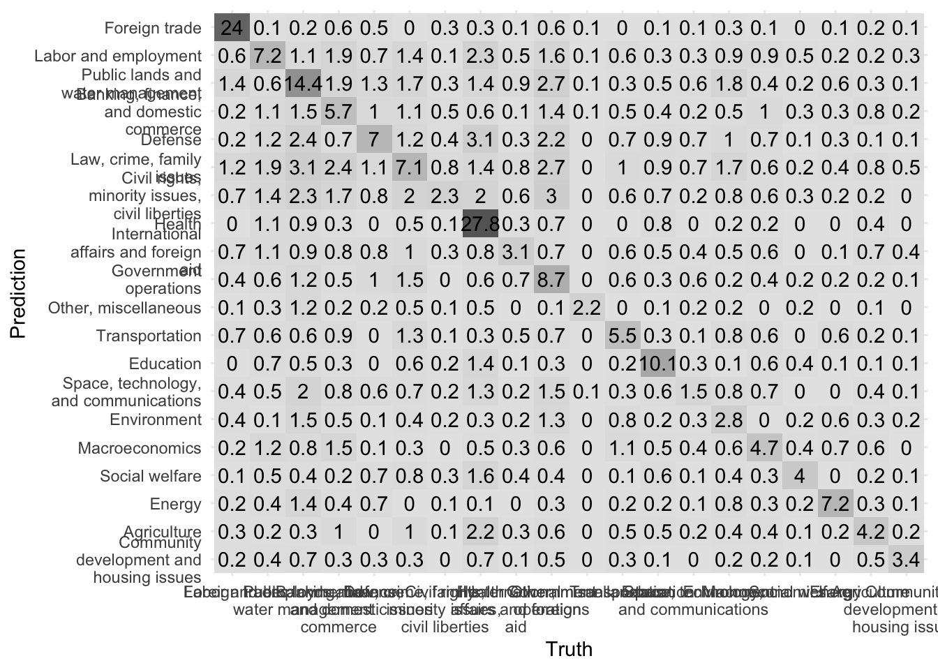
Now there are still prediction errors, but they same more evenly distributed across the matrix.
Acknowledgments
- For more detail on machine learning for text classification, see Supervised Machine Learning for Text Analysis in R by Emil Hvitfeldt and Julia Silge
Session Info
sessioninfo::session_info()
## ─ Session info ───────────────────────────────────────────────────────────────
##  setting  value
##  version  R version 4.2.1 (2022-06-23)
##  os       macOS Monterey 12.3
##  system   aarch64, darwin20
##  ui       X11
##  language (EN)
##  collate  en_US.UTF-8
##  ctype    en_US.UTF-8
##  tz       America/New_York
##  date     2022-08-22
##  pandoc   2.18 @ /Applications/RStudio.app/Contents/MacOS/quarto/bin/tools/ (via rmarkdown)
##
## ─ Packages ───────────────────────────────────────────────────────────────────
##  package       * version    date (UTC) lib source
##  assertthat      0.2.1      2019-03-21 [2] CRAN (R 4.2.0)
##  backports       1.4.1      2021-12-13 [2] CRAN (R 4.2.0)
##  blogdown        1.10       2022-05-10 [2] CRAN (R 4.2.0)
##  bookdown        0.27       2022-06-14 [2] CRAN (R 4.2.0)
##  broom         * 1.0.0      2022-07-01 [2] CRAN (R 4.2.0)
##  bslib           0.4.0      2022-07-16 [2] CRAN (R 4.2.0)
##  cachem          1.0.6      2021-08-19 [2] CRAN (R 4.2.0)
##  cellranger      1.1.0      2016-07-27 [2] CRAN (R 4.2.0)
##  class           7.3-20     2022-01-16 [2] CRAN (R 4.2.1)
##  cli             3.3.0      2022-04-25 [2] CRAN (R 4.2.0)
##  codetools       0.2-18     2020-11-04 [2] CRAN (R 4.2.1)
##  colorspace      2.0-3      2022-02-21 [2] CRAN (R 4.2.0)
##  crayon          1.5.1      2022-03-26 [2] CRAN (R 4.2.0)
##  DBI             1.1.3      2022-06-18 [2] CRAN (R 4.2.0)
##  dbplyr          2.2.1      2022-06-27 [2] CRAN (R 4.2.0)
##  dials         * 1.0.0      2022-06-14 [2] CRAN (R 4.2.0)
##  DiceDesign      1.9        2021-02-13 [2] CRAN (R 4.2.0)
##  digest          0.6.29     2021-12-01 [2] CRAN (R 4.2.0)
##  dplyr         * 1.0.9      2022-04-28 [2] CRAN (R 4.2.0)
##  ellipsis        0.3.2      2021-04-29 [2] CRAN (R 4.2.0)
##  evaluate        0.16       2022-08-09 [1] CRAN (R 4.2.1)
##  fansi           1.0.3      2022-03-24 [2] CRAN (R 4.2.0)
##  fastmap         1.1.0      2021-01-25 [2] CRAN (R 4.2.0)
##  forcats       * 0.5.1      2021-01-27 [2] CRAN (R 4.2.0)
##  foreach         1.5.2      2022-02-02 [2] CRAN (R 4.2.0)
##  fs              1.5.2      2021-12-08 [2] CRAN (R 4.2.0)
##  furrr           0.3.0      2022-05-04 [2] CRAN (R 4.2.0)
##  future          1.27.0     2022-07-22 [2] CRAN (R 4.2.0)
##  future.apply    1.9.0      2022-04-25 [2] CRAN (R 4.2.0)
##  gargle          1.2.0      2021-07-02 [2] CRAN (R 4.2.0)
##  generics        0.1.3      2022-07-05 [2] CRAN (R 4.2.0)
##  ggplot2       * 3.3.6      2022-05-03 [2] CRAN (R 4.2.0)
##  globals         0.16.0     2022-08-05 [2] CRAN (R 4.2.0)
##  glue            1.6.2      2022-02-24 [2] CRAN (R 4.2.0)
##  googledrive     2.0.0      2021-07-08 [2] CRAN (R 4.2.0)
##  googlesheets4   1.0.0      2021-07-21 [2] CRAN (R 4.2.0)
##  gower           1.0.0      2022-02-03 [2] CRAN (R 4.2.0)
##  GPfit           1.0-8      2019-02-08 [2] CRAN (R 4.2.0)
##  gtable          0.3.0      2019-03-25 [2] CRAN (R 4.2.0)
##  hardhat         1.2.0      2022-06-30 [2] CRAN (R 4.2.0)
##  haven           2.5.0      2022-04-15 [2] CRAN (R 4.2.0)
##  here            1.0.1      2020-12-13 [2] CRAN (R 4.2.0)
##  hms             1.1.1      2021-09-26 [2] CRAN (R 4.2.0)
##  htmltools       0.5.3      2022-07-18 [2] CRAN (R 4.2.0)
##  httr            1.4.3      2022-05-04 [2] CRAN (R 4.2.0)
##  infer         * 1.0.2      2022-06-10 [2] CRAN (R 4.2.0)
##  ipred           0.9-13     2022-06-02 [2] CRAN (R 4.2.0)
##  iterators       1.0.14     2022-02-05 [2] CRAN (R 4.2.0)
##  janeaustenr     0.1.5      2017-06-10 [2] CRAN (R 4.2.0)
##  jquerylib       0.1.4      2021-04-26 [2] CRAN (R 4.2.0)
##  jsonlite        1.8.0      2022-02-22 [2] CRAN (R 4.2.0)
##  knitr           1.39       2022-04-26 [2] CRAN (R 4.2.0)
##  lattice         0.20-45    2021-09-22 [2] CRAN (R 4.2.1)
##  lava            1.6.10     2021-09-02 [2] CRAN (R 4.2.0)
##  lhs             1.1.5      2022-03-22 [2] CRAN (R 4.2.0)
##  lifecycle       1.0.1      2021-09-24 [2] CRAN (R 4.2.0)
##  listenv         0.8.0      2019-12-05 [2] CRAN (R 4.2.0)
##  lubridate       1.8.0      2021-10-07 [2] CRAN (R 4.2.0)
##  magrittr        2.0.3      2022-03-30 [2] CRAN (R 4.2.0)
##  MASS            7.3-58.1   2022-08-03 [2] CRAN (R 4.2.0)
##  Matrix          1.4-1      2022-03-23 [2] CRAN (R 4.2.1)
##  modeldata     * 1.0.0      2022-07-01 [2] CRAN (R 4.2.0)
##  modelr          0.1.8      2020-05-19 [2] CRAN (R 4.2.0)
##  munsell         0.5.0      2018-06-12 [2] CRAN (R 4.2.0)
##  nnet            7.3-17     2022-01-16 [2] CRAN (R 4.2.1)
##  parallelly      1.32.1     2022-07-21 [2] CRAN (R 4.2.0)
##  parsnip       * 1.0.0      2022-06-16 [2] CRAN (R 4.2.0)
##  pillar          1.8.0      2022-07-18 [2] CRAN (R 4.2.0)
##  pkgconfig       2.0.3      2019-09-22 [2] CRAN (R 4.2.0)
##  prodlim         2019.11.13 2019-11-17 [2] CRAN (R 4.2.0)
##  purrr         * 0.3.4      2020-04-17 [2] CRAN (R 4.2.0)
##  R6              2.5.1      2021-08-19 [2] CRAN (R 4.2.0)
##  Rcpp            1.0.9      2022-07-08 [2] CRAN (R 4.2.0)
##  readr         * 2.1.2      2022-01-30 [2] CRAN (R 4.2.0)
##  readxl          1.4.0      2022-03-28 [2] CRAN (R 4.2.0)
##  recipes       * 1.0.1      2022-07-07 [2] CRAN (R 4.2.0)
##  reprex          2.0.1.9000 2022-08-10 [1] Github (tidyverse/reprex@6d3ad07)
##  rlang           1.0.4      2022-07-12 [2] CRAN (R 4.2.0)
##  rmarkdown       2.14       2022-04-25 [2] CRAN (R 4.2.0)
##  rpart           4.1.16     2022-01-24 [2] CRAN (R 4.2.1)
##  rprojroot       2.0.3      2022-04-02 [2] CRAN (R 4.2.0)
##  rsample       * 1.1.0      2022-08-08 [2] CRAN (R 4.2.1)
##  rstudioapi      0.13       2020-11-12 [2] CRAN (R 4.2.0)
##  rvest           1.0.2      2021-10-16 [2] CRAN (R 4.2.0)
##  sass            0.4.2      2022-07-16 [2] CRAN (R 4.2.0)
##  scales        * 1.2.0      2022-04-13 [2] CRAN (R 4.2.0)
##  sessioninfo     1.2.2      2021-12-06 [2] CRAN (R 4.2.0)
##  SnowballC       0.7.0      2020-04-01 [2] CRAN (R 4.2.0)
##  stringi         1.7.8      2022-07-11 [2] CRAN (R 4.2.0)
##  stringr       * 1.4.0      2019-02-10 [2] CRAN (R 4.2.0)
##  survival        3.3-1      2022-03-03 [2] CRAN (R 4.2.1)
##  tibble        * 3.1.8      2022-07-22 [2] CRAN (R 4.2.0)
##  tidymodels    * 1.0.0      2022-07-13 [2] CRAN (R 4.2.0)
##  tidyr         * 1.2.0      2022-02-01 [2] CRAN (R 4.2.0)
##  tidyselect      1.1.2      2022-02-21 [2] CRAN (R 4.2.0)
##  tidytext      * 0.3.3      2022-05-09 [2] CRAN (R 4.2.0)
##  tidyverse     * 1.3.2      2022-07-18 [2] CRAN (R 4.2.0)
##  timeDate        4021.104   2022-07-19 [2] CRAN (R 4.2.0)
##  tokenizers      0.2.1      2018-03-29 [2] CRAN (R 4.2.0)
##  tune          * 1.0.0      2022-07-07 [2] CRAN (R 4.2.0)
##  tzdb            0.3.0      2022-03-28 [2] CRAN (R 4.2.0)
##  utf8            1.2.2      2021-07-24 [2] CRAN (R 4.2.0)
##  vctrs           0.4.1      2022-04-13 [2] CRAN (R 4.2.0)
##  withr           2.5.0      2022-03-03 [2] CRAN (R 4.2.0)
##  workflows     * 1.0.0      2022-07-05 [2] CRAN (R 4.2.0)
##  workflowsets  * 1.0.0      2022-07-12 [2] CRAN (R 4.2.0)
##  xfun            0.31       2022-05-10 [1] CRAN (R 4.2.0)
##  xml2            1.3.3      2021-11-30 [2] CRAN (R 4.2.0)
##  yaml            2.3.5      2022-02-21 [2] CRAN (R 4.2.0)
##  yardstick     * 1.0.0      2022-06-06 [2] CRAN (R 4.2.0)
##
##  [1] /Users/soltoffbc/Library/R/arm64/4.2/library
##  [2] /Library/Frameworks/R.framework/Versions/4.2-arm64/Resources/library
##
## ──────────────────────────────────────────────────────────────────────────────