Practicing tidytext with song titles
library(tidyverse)
library(acs)
library(tidytext)
library(here)

set.seed(1234)
theme_set(theme_minimal())
Run the code below in your console to download this exercise as a set of R scripts.
usethis::use_course("cis-ds/text-analysis-fundamentals-and-sentiment-analysis")
Today let’s practice our tidytext skills with a basic analysis of song titles. That is, how often is each U.S. state mentioned in a popular song? We’ll define popular songs as those in Billboard’s Year-End Hot 100 from 1958 to the present.
Download population data for U.S. states
First let’s use the tidycensus package to access the U.S. Census Bureau API and obtain population numbers for each state in 2016. This will help us later to normalize state mentions based on relative population size.1
To import the data in-class, run:
pop_df <- read_csv("http://info5940.infosci.cornell.edu/data/pop2016.csv")
The code below shows how the file was originally constructed.
# retrieve state populations in 2016 from Census Bureau ACS
library(tidycensus)
pop_df <- get_acs(
  geography = "state", year = 2016,
  variables = c(population = "B01003_001")
) %>%
  # remove moe and tidy the data frame
  select(-moe) %>%
  spread(variable, estimate) %>%
  # clean the data to match with the structure of the lyrics data
  rename(state_name = NAME) %>%
  mutate(state_name = str_to_lower(state_name)) %>%
  filter(state_name != "Puerto Rico") %>%
  write_csv(here("static", "data", "pop2016.csv"))
## Getting data from the 2012-2016 5-year ACS
# do these results make sense?
pop_df %>%
  arrange(desc(population)) %>%
  top_n(10)
## Selecting by population
## # A tibble: 10 × 3
##    GEOID state_name     population
##    <chr> <chr>               <dbl>
##  1 06    california       38654206
##  2 48    texas            26956435
##  3 12    florida          19934451
##  4 36    new york         19697457
##  5 17    illinois         12851684
##  6 42    pennsylvania     12783977
##  7 39    ohio             11586941
##  8 13    georgia          10099320
##  9 37    north carolina    9940828
## 10 26    michigan          9909600
Retrieve song lyrics
Next we need to retrieve the song lyrics for all our songs. Kaylin Walker provides a GitHub repo with the necessary files.
To import the data in-class, use
song_lyrics <- read_csv("http://info5940.infosci.cornell.edu/data/billboard_lyrics_1964-2015.csv")
## Rows: 5100 Columns: 6
## ── Column specification ────────────────────────────────────────────────────────
## Delimiter: ","
## chr (3): Song, Artist, Lyrics
## dbl (3): Rank, Year, Source
##
## ℹ Use `spec()` to retrieve the full column specification for this data.
## ℹ Specify the column types or set `show_col_types = FALSE` to quiet this message.
## Rows: 5,100
## Columns: 6
## $ Rank   <dbl> 1, 2, 3, 4, 5, 6, 7, 8, 9, 10, 11, 12, 13, 14, 15, 16, 17, 18, …
## $ Song   <chr> "wooly bully", "i cant help myself sugar pie honey bunch", "i c…
## $ Artist <chr> "sam the sham and the pharaohs", "four tops", "the rolling ston…
## $ Year   <dbl> 1965, 1965, 1965, 1965, 1965, 1965, 1965, 1965, 1965, 1965, 196…
## $ Lyrics <chr> "sam the sham miscellaneous wooly bully wooly bully sam the sha…
## $ Source <dbl> 3, 1, 1, 1, 1, 1, 3, 5, 1, 3, 3, 1, 3, 1, 3, 3, 3, 3, 1, 1, 1, …
The lyrics are stored as character vectors, one string for each song. Consider the song Uptown Funk:
## this hit that ice cold michelle pfeiffer that white gold this one for them hood
## girls them good girls straight masterpieces stylin whilen livin it up in the
## city got chucks on with saint laurent got kiss myself im so prettyim too hot
## hot damn called a police and a fireman im too hot hot damn make a dragon wanna
## retire man im too hot hot damn say my name you know who i am im too hot hot damn
## am i bad bout that money break it downgirls hit your hallelujah whoo girls hit
## your hallelujah whoo girls hit your hallelujah whoo cause uptown funk gon give
## it to you cause uptown funk gon give it to you cause uptown funk gon give it
## to you saturday night and we in the spot dont believe me just watch come ondont
## believe me just watch uhdont believe me just watch dont believe me just watch
## dont believe me just watch dont believe me just watch hey hey hey oh meaning
## byamandah editor 70s girl group the sequence accused bruno mars and producer
## mark ronson of ripping their sound off in uptown funk their song in question is
## funk you see all stop wait a minute fill my cup put some liquor in it take a sip
## sign a check julio get the stretch ride to harlem hollywood jackson mississippi
## if we show up we gon show out smoother than a fresh jar of skippyim too hot
## hot damn called a police and a fireman im too hot hot damn make a dragon wanna
## retire man im too hot hot damn bitch say my name you know who i am im too hot
## hot damn am i bad bout that money break it downgirls hit your hallelujah whoo
## girls hit your hallelujah whoo girls hit your hallelujah whoo cause uptown funk
## gon give it to you cause uptown funk gon give it to you cause uptown funk gon
## give it to you saturday night and we in the spot dont believe me just watch
## come ondont believe me just watch uhdont believe me just watch uh dont believe
## me just watch uh dont believe me just watch dont believe me just watch hey hey
## hey ohbefore we leave lemmi tell yall a lil something uptown funk you up uptown
## funk you up uptown funk you up uptown funk you up uh i said uptown funk you up
## uptown funk you up uptown funk you up uptown funk you upcome on dance jump on
## it if you sexy then flaunt it if you freaky then own it dont brag about it come
## show mecome on dance jump on it if you sexy then flaunt it well its saturday
## night and we in the spot dont believe me just watch come ondont believe me just
## watch uhdont believe me just watch uh dont believe me just watch uh dont believe
## me just watch dont believe me just watch hey hey hey ohuptown funk you up uptown
## funk you up say what uptown funk you up uptown funk you up uptown funk you up
## uptown funk you up say what uptown funk you up uptown funk you up uptown funk
## you up uptown funk you up say what uptown funk you up uptown funk you up uptown
## funk you up uptown funk you up say what uptown funk you up
Find and visualize the state names in the song lyrics
Now your work begins!
Use tidytext to create a data frame with one row for each token in each song
Hint: To search for matching state names, this data frame should include both unigrams and bi-grams.
Click for the solution
# tokenize
lyrics_unigrams <- unnest_tokens(
  tbl = song_lyrics,
  output = word,
  input = Lyrics
)
lyrics_bigrams <- unnest_tokens(
  tbl = song_lyrics,
  output = word,
  input = Lyrics,
  token = "ngrams", n = 2
)

# combine together
tidy_lyrics <- bind_rows(lyrics_unigrams, lyrics_bigrams)
tidy_lyrics
## # A tibble: 3,201,465 × 6
##     Rank Song        Artist                         Year Source word
##    <dbl> <chr>       <chr>                         <dbl>  <dbl> <chr>
##  1     1 wooly bully sam the sham and the pharaohs  1965      3 sam
##  2     1 wooly bully sam the sham and the pharaohs  1965      3 the
##  3     1 wooly bully sam the sham and the pharaohs  1965      3 sham
##  4     1 wooly bully sam the sham and the pharaohs  1965      3 miscellaneous
##  5     1 wooly bully sam the sham and the pharaohs  1965      3 wooly
##  6     1 wooly bully sam the sham and the pharaohs  1965      3 bully
##  7     1 wooly bully sam the sham and the pharaohs  1965      3 wooly
##  8     1 wooly bully sam the sham and the pharaohs  1965      3 bully
##  9     1 wooly bully sam the sham and the pharaohs  1965      3 sam
## 10     1 wooly bully sam the sham and the pharaohs  1965      3 the
## # … with 3,201,455 more rows
## # ℹ Use `print(n = ...)` to see more rows
The variable word in this data frame contains all the possible words and bigrams that might be state names in all the lyrics.
Find all the state names occurring in the song lyrics
First create a data frame that meets this criteria, then save a new data frame that only includes one observation for each matching song. That is, if the song is “New York, New York”, there should only be one row in the resulting table for that song.
Click for the solution
inner_join(tidy_lyrics, pop_df, by = c("word" = "state_name"))
## # A tibble: 526 × 8
## Rank Song Artist Year Source word GEOID popul…¹
## <dbl> <chr> <chr> <dbl> <dbl> <chr> <chr> <dbl>
## 1 12 king of the road roger miller 1965 1 maine 23 1.33e6
## 2 29 eve of destruction barry mcguire 1965 1 alabama 01 4.84e6
## 3 49 california girls the beach boys 1965 3 california 06 3.87e7
## 4 49 california girls the beach boys 1965 3 california 06 3.87e7
## 5 49 california girls the beach boys 1965 3 california 06 3.87e7
## 6 49 california girls the beach boys 1965 3 california 06 3.87e7
## 7 49 california girls the beach boys 1965 3 california 06 3.87e7
## 8 49 california girls the beach boys 1965 3 california 06 3.87e7
## 9 49 california girls the beach boys 1965 3 california 06 3.87e7
## 10 49 california girls the beach boys 1965 3 california 06 3.87e7
## # … with 516 more rows, and abbreviated variable name ¹population
## # ℹ Use `print(n = ...)` to see more rows
Let’s only count each state once per song that it is mentioned in.
tidy_lyrics <- inner_join(tidy_lyrics, pop_df, by = c("word" = "state_name")) %>%
  distinct(Rank, Song, Artist, Year, word, .keep_all = TRUE)
tidy_lyrics
## # A tibble: 253 × 8
## Rank Song Artist Year Source word GEOID popul…¹
## <dbl> <chr> <chr> <dbl> <dbl> <chr> <chr> <dbl>
## 1 12 king of the road roger m… 1965 1 maine 23 1.33e6
## 2 29 eve of destruction barry m… 1965 1 alab… 01 4.84e6
## 3 49 california girls the bea… 1965 3 cali… 06 3.87e7
## 4 10 california dreamin the mam… 1966 3 cali… 06 3.87e7
## 5 77 message to michael dionne … 1966 1 kent… 21 4.41e6
## 6 61 california nights lesley … 1967 1 cali… 06 3.87e7
## 7 4 sittin on the dock of the bay otis re… 1968 1 geor… 13 1.01e7
## 8 10 tighten up archie … 1968 3 texas 48 2.70e7
## 9 25 get back the bea… 1969 3 ariz… 04 6.73e6
## 10 25 get back the bea… 1969 3 cali… 06 3.87e7
## # … with 243 more rows, and abbreviated variable name ¹population
## # ℹ Use `print(n = ...)` to see more rows
Calculate the frequency for each state’s mention in a song and create a new column for the frequency adjusted by the state’s population
Click for the solution
(state_counts <- tidy_lyrics %>%
  count(word) %>%
  arrange(desc(n)))
## # A tibble: 33 × 2
##    word            n
##    <chr>       <int>
##  1 new york       64
##  2 california     34
##  3 georgia        22
##  4 tennessee      14
##  5 texas          14
##  6 alabama        12
##  7 mississippi    10
##  8 kentucky        7
##  9 hawaii          6
## 10 illinois        6
## # … with 23 more rows
## # ℹ Use `print(n = ...)` to see more rows
pop_df <- pop_df %>%
  left_join(state_counts, by = c("state_name" = "word")) %>%
  mutate(rate = n / population * 1e6)

## which are the top ten states by rate?
pop_df %>%
  arrange(desc(rate)) %>%
  top_n(10)
## Selecting by rate
## # A tibble: 10 × 5
##    GEOID state_name  population     n  rate
##    <chr> <chr>            <dbl> <int> <dbl>
##  1 15    hawaii         1413673     6  4.24
##  2 28    mississippi    2989192    10  3.35
##  3 36    new york      19697457    64  3.25
##  4 01    alabama        4841164    12  2.48
##  5 23    maine          1329923     3  2.26
##  6 13    georgia       10099320    22  2.18
##  7 47    tennessee      6548009    14  2.14
##  8 30    montana        1023391     2  1.95
##  9 31    nebraska       1881259     3  1.59
## 10 21    kentucky       4411989     7  1.59
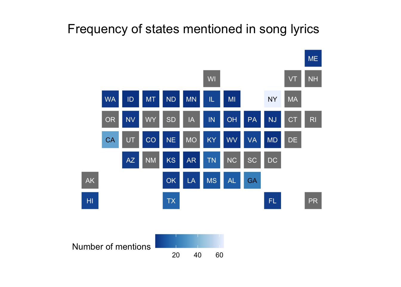
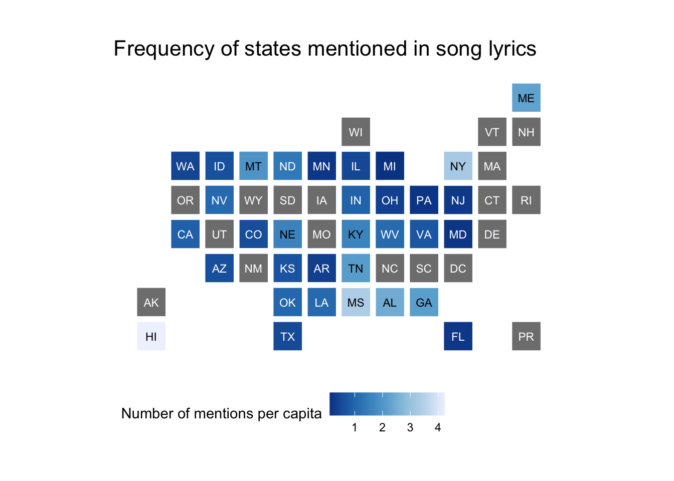
Make a choropleth map for both the raw frequency counts and relative frequency counts
The statebins package is a nifty shortcut for making basic U.S. cartogram maps.
library(statebins)

pop_df %>%
  mutate(
    state_name = stringr::str_to_title(state_name),
    state_name = if_else(state_name == "District Of Columbia",
      "District of Columbia", state_name
    )
  ) %>%
  statebins(
    state_col = "state_name", value_col = "n",
    name = "Number of mentions"
  ) +
  labs(title = "Frequency of states mentioned in song lyrics") +
  theme_statebins()
pop_df %>%
  mutate(
    state_name = stringr::str_to_title(state_name),
    state_name = if_else(state_name == "District Of Columbia",
      "District of Columbia", state_name
    )
  ) %>%
  statebins(
    state_col = "state_name", value_col = "rate",
    name = "Number of mentions per capita"
  ) +
  labs(title = "Frequency of states mentioned in song lyrics") +
  theme_statebins()
Acknowledgments
- This page is derived in part from SONG LYRICS ACROSS THE UNITED STATES and licensed under a Creative Commons Attribution-ShareAlike 4.0 International License.
Session Info
sessioninfo::session_info()
## ─ Session info ───────────────────────────────────────────────────────────────
##  setting  value
##  version  R version 4.2.1 (2022-06-23)
##  os       macOS Monterey 12.3
##  system   aarch64, darwin20
##  ui       X11
##  language (EN)
##  collate  en_US.UTF-8
##  ctype    en_US.UTF-8
##  tz       America/New_York
##  date     2022-08-22
##  pandoc   2.18 @ /Applications/RStudio.app/Contents/MacOS/quarto/bin/tools/ (via rmarkdown)
##
## ─ Packages ───────────────────────────────────────────────────────────────────
##  package       * version    date (UTC) lib source
##  acs           * 2.1.4      2019-02-19 [2] CRAN (R 4.2.0)
##  assertthat      0.2.1      2019-03-21 [2] CRAN (R 4.2.0)
##  backports       1.4.1      2021-12-13 [2] CRAN (R 4.2.0)
##  blogdown        1.10       2022-05-10 [2] CRAN (R 4.2.0)
##  bookdown        0.27       2022-06-14 [2] CRAN (R 4.2.0)
##  broom           1.0.0      2022-07-01 [2] CRAN (R 4.2.0)
##  bslib           0.4.0      2022-07-16 [2] CRAN (R 4.2.0)
##  cachem          1.0.6      2021-08-19 [2] CRAN (R 4.2.0)
##  cellranger      1.1.0      2016-07-27 [2] CRAN (R 4.2.0)
##  cli             3.3.0      2022-04-25 [2] CRAN (R 4.2.0)
##  colorspace      2.0-3      2022-02-21 [2] CRAN (R 4.2.0)
##  crayon          1.5.1      2022-03-26 [2] CRAN (R 4.2.0)
##  DBI             1.1.3      2022-06-18 [2] CRAN (R 4.2.0)
##  dbplyr          2.2.1      2022-06-27 [2] CRAN (R 4.2.0)
##  digest          0.6.29     2021-12-01 [2] CRAN (R 4.2.0)
##  dplyr         * 1.0.9      2022-04-28 [2] CRAN (R 4.2.0)
##  ellipsis        0.3.2      2021-04-29 [2] CRAN (R 4.2.0)
##  evaluate        0.16       2022-08-09 [1] CRAN (R 4.2.1)
##  fansi           1.0.3      2022-03-24 [2] CRAN (R 4.2.0)
##  fastmap         1.1.0      2021-01-25 [2] CRAN (R 4.2.0)
##  forcats       * 0.5.1      2021-01-27 [2] CRAN (R 4.2.0)
##  fs              1.5.2      2021-12-08 [2] CRAN (R 4.2.0)
##  gargle          1.2.0      2021-07-02 [2] CRAN (R 4.2.0)
##  generics        0.1.3      2022-07-05 [2] CRAN (R 4.2.0)
##  ggplot2       * 3.3.6      2022-05-03 [2] CRAN (R 4.2.0)
##  glue            1.6.2      2022-02-24 [2] CRAN (R 4.2.0)
##  googledrive     2.0.0      2021-07-08 [2] CRAN (R 4.2.0)
##  googlesheets4   1.0.0      2021-07-21 [2] CRAN (R 4.2.0)
##  gtable          0.3.0      2019-03-25 [2] CRAN (R 4.2.0)
##  haven           2.5.0      2022-04-15 [2] CRAN (R 4.2.0)
##  here          * 1.0.1      2020-12-13 [2] CRAN (R 4.2.0)
##  hms             1.1.1      2021-09-26 [2] CRAN (R 4.2.0)
##  htmltools       0.5.3      2022-07-18 [2] CRAN (R 4.2.0)
##  httr            1.4.3      2022-05-04 [2] CRAN (R 4.2.0)
##  janeaustenr     0.1.5      2017-06-10 [2] CRAN (R 4.2.0)
##  jquerylib       0.1.4      2021-04-26 [2] CRAN (R 4.2.0)
##  jsonlite        1.8.0      2022-02-22 [2] CRAN (R 4.2.0)
##  knitr           1.39       2022-04-26 [2] CRAN (R 4.2.0)
##  lattice         0.20-45    2021-09-22 [2] CRAN (R 4.2.1)
##  lifecycle       1.0.1      2021-09-24 [2] CRAN (R 4.2.0)
##  lubridate       1.8.0      2021-10-07 [2] CRAN (R 4.2.0)
##  magrittr        2.0.3      2022-03-30 [2] CRAN (R 4.2.0)
##  Matrix          1.4-1      2022-03-23 [2] CRAN (R 4.2.1)
##  modelr          0.1.8      2020-05-19 [2] CRAN (R 4.2.0)
##  munsell         0.5.0      2018-06-12 [2] CRAN (R 4.2.0)
##  pillar          1.8.0      2022-07-18 [2] CRAN (R 4.2.0)
##  pkgconfig       2.0.3      2019-09-22 [2] CRAN (R 4.2.0)
##  plyr            1.8.7      2022-03-24 [2] CRAN (R 4.2.0)
##  purrr         * 0.3.4      2020-04-17 [2] CRAN (R 4.2.0)
##  R6              2.5.1      2021-08-19 [2] CRAN (R 4.2.0)
##  Rcpp            1.0.9      2022-07-08 [2] CRAN (R 4.2.0)
##  readr         * 2.1.2      2022-01-30 [2] CRAN (R 4.2.0)
##  readxl          1.4.0      2022-03-28 [2] CRAN (R 4.2.0)
##  reprex          2.0.1.9000 2022-08-10 [1] Github (tidyverse/reprex@6d3ad07)
##  rlang           1.0.4      2022-07-12 [2] CRAN (R 4.2.0)
##  rmarkdown       2.14       2022-04-25 [2] CRAN (R 4.2.0)
##  rprojroot       2.0.3      2022-04-02 [2] CRAN (R 4.2.0)
##  rstudioapi      0.13       2020-11-12 [2] CRAN (R 4.2.0)
##  rvest           1.0.2      2021-10-16 [2] CRAN (R 4.2.0)
##  sass            0.4.2      2022-07-16 [2] CRAN (R 4.2.0)
##  scales          1.2.0      2022-04-13 [2] CRAN (R 4.2.0)
##  sessioninfo     1.2.2      2021-12-06 [2] CRAN (R 4.2.0)
##  SnowballC       0.7.0      2020-04-01 [2] CRAN (R 4.2.0)
##  stringi         1.7.8      2022-07-11 [2] CRAN (R 4.2.0)
##  stringr       * 1.4.0      2019-02-10 [2] CRAN (R 4.2.0)
##  tibble        * 3.1.8      2022-07-22 [2] CRAN (R 4.2.0)
##  tidyr         * 1.2.0      2022-02-01 [2] CRAN (R 4.2.0)
##  tidyselect      1.1.2      2022-02-21 [2] CRAN (R 4.2.0)
##  tidytext      * 0.3.3      2022-05-09 [2] CRAN (R 4.2.0)
##  tidyverse     * 1.3.2      2022-07-18 [2] CRAN (R 4.2.0)
##  tokenizers      0.2.1      2018-03-29 [2] CRAN (R 4.2.0)
##  tzdb            0.3.0      2022-03-28 [2] CRAN (R 4.2.0)
##  utf8            1.2.2      2021-07-24 [2] CRAN (R 4.2.0)
##  vctrs           0.4.1      2022-04-13 [2] CRAN (R 4.2.0)
##  withr           2.5.0      2022-03-03 [2] CRAN (R 4.2.0)
##  xfun            0.31       2022-05-10 [1] CRAN (R 4.2.0)
##  XML           * 3.99-0.10  2022-06-09 [2] CRAN (R 4.2.0)
##  xml2            1.3.3      2021-11-30 [2] CRAN (R 4.2.0)
##  yaml            2.3.5      2022-02-21 [2] CRAN (R 4.2.0)
##
##  [1] /Users/soltoffbc/Library/R/arm64/4.2/library
##  [2] /Library/Frameworks/R.framework/Versions/4.2-arm64/Resources/library
##
## ──────────────────────────────────────────────────────────────────────────────
For instance, California has a lot more people than Rhode Island so it makes sense that California would be mentioned more often in popular songs. But per capita, are these mentions different? ↩︎