Predicting song artist from lyrics
library(tidyverse)
library(tidymodels)
library(here)
library(stringr)
library(textrecipes)
library(themis)
library(vip)

set.seed(123)
theme_set(theme_minimal())
Run the code below in your console to download this exercise as a set of R scripts.
usethis::use_course("cis-ds/text-analysis-classification-and-topic-modeling")
Beyoncé and Taylor Swift are two iconic singer/songwriters from the past twenty years. While they have achieved worldwide recognition for their contributions to music, they also have quite diverse musical genres and themes. For example, much of Taylor Swift’s early work is commonly associated with love and heartbreak, while Beyoncé’s career has been noted for many compositions surrounding female-empowerment. Based purely on the lyrics, can we predict if a song is by Beyoncé or Taylor Swift?
Import data
Our data comes from #TidyTuesday which compiled individual song lyrics from each singer’s discography as of September 29, 2020. Here we import the data files and do some light cleaning to standardize each file.1
# get beyonce and taylor swift lyrics
beyonce_lyrics <- read_csv("https://raw.githubusercontent.com/rfordatascience/tidytuesday/master/data/2020/2020-09-29/beyonce_lyrics.csv")
## Rows: 22616 Columns: 6
## ── Column specification ────────────────────────────────────────────────────────
## Delimiter: ","
## chr (3): line, song_name, artist_name
## dbl (3): song_id, artist_id, song_line
##
## ℹ Use `spec()` to retrieve the full column specification for this data.
## ℹ Specify the column types or set `show_col_types = FALSE` to quiet this message.
taylor_swift_lyrics <- read_csv("https://raw.githubusercontent.com/rfordatascience/tidytuesday/master/data/2020/2020-09-29/taylor_swift_lyrics.csv")
## Rows: 132 Columns: 4
## ── Column specification ────────────────────────────────────────────────────────
## Delimiter: ","
## chr (4): Artist, Album, Title, Lyrics
##
## ℹ Use `spec()` to retrieve the full column specification for this data.
## ℹ Specify the column types or set `show_col_types = FALSE` to quiet this message.
extra_lyrics <- read_csv(here("static", "data", "updated-album-lyrics.csv"))
## Rows: 2563 Columns: 4
## ── Column specification ────────────────────────────────────────────────────────
## Delimiter: ","
## chr (4): Artist, Album, Title, Lyrics
##
## ℹ Use `spec()` to retrieve the full column specification for this data.
## ℹ Specify the column types or set `show_col_types = FALSE` to quiet this message.
# clean lyrics for binding
beyonce_clean <- bind_rows(
  beyonce_lyrics,
  extra_lyrics
  ) %>%
  # convert to one row per song
  group_by(song_id, song_name, artist_name) %>%
  summarize(Lyrics = str_flatten(line, collapse = " ")) %>%
  ungroup() %>%
  # clean column names
  select(artist = artist_name, song_title = song_name, lyrics = Lyrics)
## `summarise()` has grouped output by 'song_id', 'song_name'. You can override
## using the `.groups` argument.
taylor_swift_clean <- taylor_swift_lyrics %>%
  # clean column names
  select(artist = Artist, song_title = Title, lyrics = Lyrics)

# combine into single data file
lyrics <- bind_rows(beyonce_clean, taylor_swift_clean) %>%
  mutate(artist = factor(artist)) %>%
  drop_na()
lyrics
## # A tibble: 523 × 3
##    artist  song_title                                                     lyrics
##    <fct>   <chr>                                                          <chr>
##  1 Beyoncé Ego (Remix) (Ft. Kanye West)                                   "I go…
##  2 Beyoncé Irreplaceable (Rap Version) (Ft. Ghostface Killah)             "To t…
##  3 Beyoncé Smash Into You                                                 "Head…
##  4 Beyoncé Cards Never Lie (Ft. Rah Digga & Wyclef Jean)                  "The …
##  5 Beyoncé If Looks Could Kill (You Would Be Dead) (Ft. Sam Sarpong & Ya… "Swee…
##  6 Beyoncé The Last Great Seduction (Ft. Mekhi Phifer)                    "You …
##  7 Beyoncé Check on It (LP Version) (Ft. Slim Thug)                       "Swiz…
##  8 Beyoncé Crazy in Love (Ft. JAY-Z)                                      "Yes!…
##  9 Beyoncé Déjà Vu (Ft. JAY-Z)                                            "Bass…
## 10 Beyoncé Me, Myself & I (Remix) (Ft. Ghostface Killah)                  "Ahh,…
## # … with 513 more rows
Preprocess the dataset for modeling
Resampling folds
- Split the data into training/test sets with 75% allocated for training
- Split the training set into 10 cross-validation folds
Click for the solution
rsample is the go-to package for this resampling.
# split into training/testing
set.seed(123)
lyrics_split <- initial_split(data = lyrics, strata = artist, prop = 0.75)

lyrics_train <- training(lyrics_split)
lyrics_test <- testing(lyrics_split)

# create cross-validation folds
lyrics_folds <- vfold_cv(data = lyrics_train, strata = artist)
Define the feature engineering recipe
Define a feature engineering recipe to predict the song’s artist as a function of the lyrics
Tokenize the song lyrics
Remove stop words
Only keep the 500 most frequently appearing tokens
Calculate tf-idf scores for the remaining tokens
This will generate one column for every token. Each column will have the standardized name
tfidf_lyrics_*where*is the specific token. Instead we would prefer the column names simply be*. You can remove thetfidf_lyrics_prefix using# Simplify these names step_rename_at(starts_with("tfidf_lyrics_"), fn = ~ str_replace_all( string = ., pattern = "tfidf_lyrics_", replacement = "" ) )
Downsample the observations so there are an equal number of songs by Beyoncé and Taylor Swift in the analysis set
Click for the solution
# define preprocessing recipe
lyrics_rec <- recipe(artist ~ lyrics, data = lyrics_train) %>%
step_tokenize(lyrics) %>%
step_stopwords(lyrics) %>%
step_tokenfilter(lyrics, max_tokens = 500) %>%
step_tfidf(lyrics) %>%
# Simplify these names
step_rename_at(starts_with("tfidf_lyrics_"),
  fn = ~ str_replace_all(
    string = .,
    pattern = "tfidf_lyrics_",
    replacement = ""
  )
) %>%
step_downsample(artist)
lyrics_rec
## Recipe
##
## Inputs:
##
##       role #variables
##    outcome          1
##  predictor          1
##
## Operations:
##
## Tokenization for lyrics
## Stop word removal for lyrics
## Text filtering for lyrics
## Term frequency-inverse document frequency with lyrics
## Variable renaming for starts_with("tfidf_lyrics_")
## Down-sampling based on artist
Estimate a random forest model
- Define a random forest model grown with 1000 trees using the
rangerengine. - Define a workflow using the feature engineering recipe and random forest model specification. Fit the workflow using the cross-validation folds.
- Use
control = control_resamples(save_pred = TRUE)to save the assessment set predictions. We need these to assess the model’s performance.
- Use
Click for the solution
# define the model specification
ranger_spec <- rand_forest(trees = 1000) %>%
  set_mode("classification") %>%
  set_engine("ranger")

# define the workflow
ranger_workflow <- workflow() %>%
  add_recipe(lyrics_rec) %>%
  add_model(ranger_spec)

# fit the model to each of the cross-validation folds
ranger_cv <- ranger_workflow %>%
  fit_resamples(
    resamples = lyrics_folds,
    control = control_resamples(save_pred = TRUE)
  )
Evaluate model performance
- Calculate the model’s accuracy and ROC AUC. How did it perform?
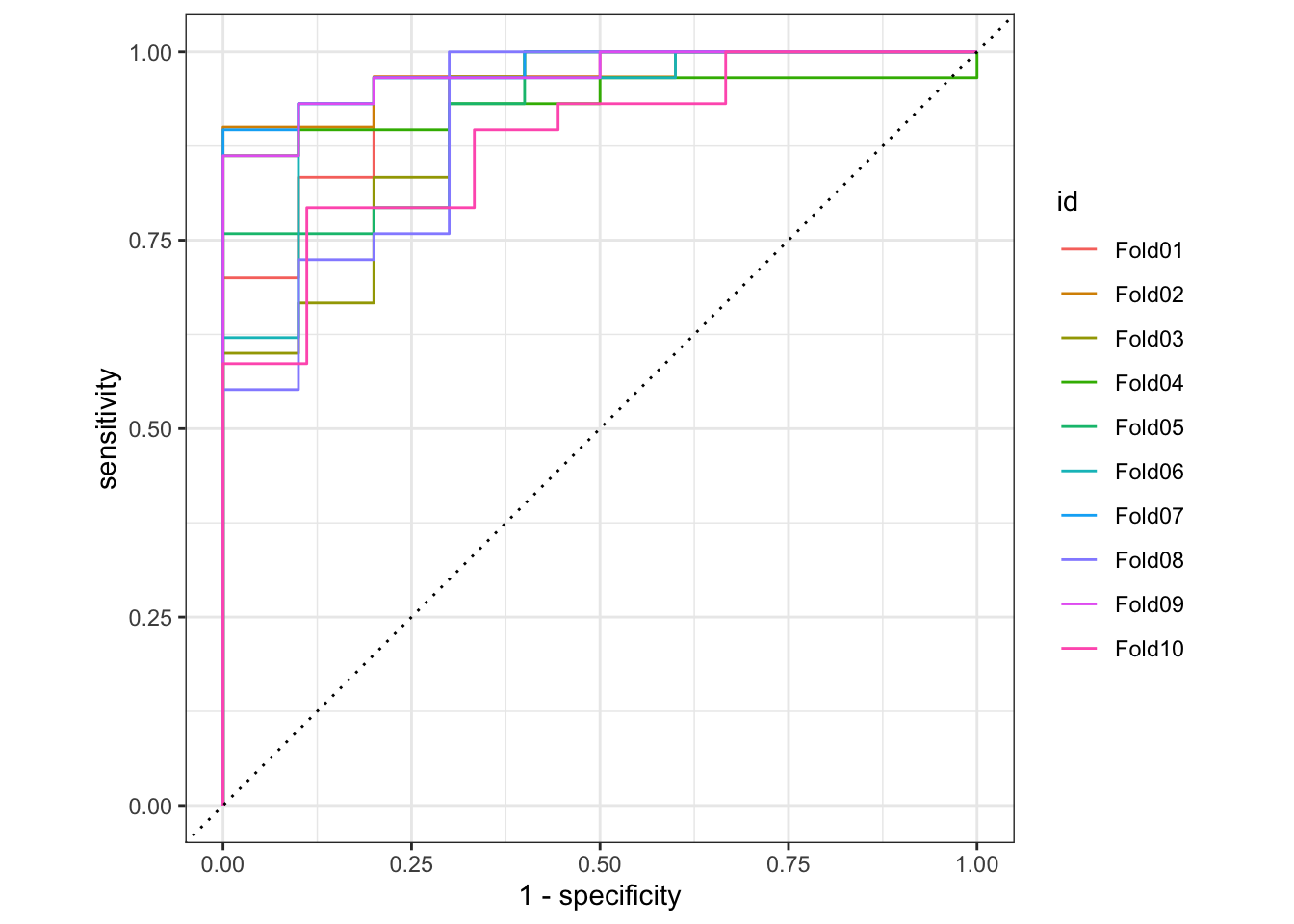
- Draw the ROC curve for each validation fold
- Generate the resampled confusion matrix for the model and draw it using a heatmap. How does the model perform predicting Beyoncé songs relative to Taylor Swift songs?
Click for the solution
# extract metrics and predictions
ranger_cv_metrics <- collect_metrics(ranger_cv)
ranger_cv_predictions <- collect_predictions(ranger_cv)

# how well did the model perform?
ranger_cv_metrics
## # A tibble: 2 × 6
##   .metric  .estimator  mean     n std_err .config
##   <chr>    <chr>      <dbl> <int>   <dbl> <chr>
## 1 accuracy binary     0.826    10 0.0232  Preprocessor1_Model1
## 2 roc_auc  binary     0.935    10 0.00986 Preprocessor1_Model1
# roc curve
ranger_cv_predictions %>%
  group_by(id) %>%
  roc_curve(truth = artist, .pred_Beyoncé) %>%
  autoplot()
# confusion matrix
conf_mat_resampled(x = ranger_cv, tidy = FALSE) %>%
  autoplot(type = "heatmap")
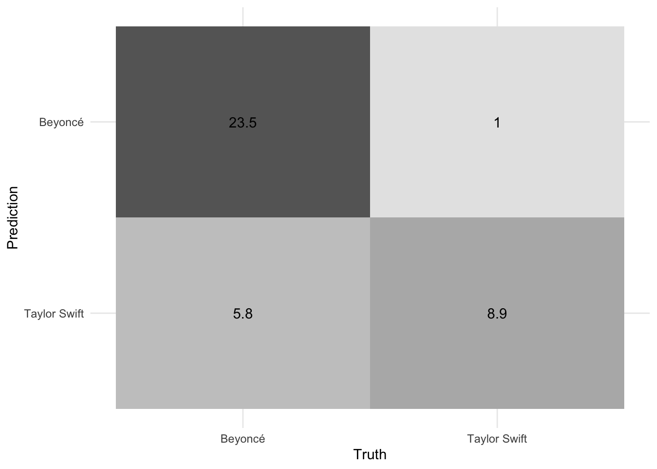
Overall the random forest model is reasonable at distinguishing Beyoncé from Taylor Swift based purely on the lyrics. A ROC AUC value of 0.93 is pretty good for a binary classification task. We can also see the model more accurately predicts Beyoncé’s songs compared to Taylor Swift. Part of this is because Beyoncé’s catalog is much larger (392 songs compared to only 132 for Taylor Swift), but this should have been accounted for through the downsampling. Even after this procedure, the model still has better sensitivity to Beyoncé.
Penalized regression
Define the feature engineering recipe
Define the same feature engineering recipe as before, with two adjustments:
- Calculate all possible 1-grams, 2-grams, 3-grams, 4-grams, and 5-grams
- Retain the 2000 most frequently occurring tokens.
Click for the solution
# redefine recipe to include multiple n-grams
glmnet_rec <- recipe(artist ~ lyrics, data = lyrics_train) %>%
  step_tokenize(lyrics) %>%
  step_stopwords(lyrics) %>%
  step_ngram(lyrics, num_tokens = 5L, min_num_tokens = 1L) %>%
  step_tokenfilter(lyrics, max_tokens = 2000) %>%
  step_tfidf(lyrics) %>%
  # Simplify these names
  step_rename_at(starts_with("tfidf_lyrics_"),
    fn = ~ str_replace_all(string = ., pattern = "tfidf_lyrics_", replacement = "")
  ) %>%
  step_downsample(artist)
glmnet_rec
## Recipe
##
## Inputs:
##
##       role #variables
##    outcome          1
##  predictor          1
##
## Operations:
##
## Tokenization for lyrics
## Stop word removal for lyrics
## ngramming for lyrics
## Text filtering for lyrics
## Term frequency-inverse document frequency with lyrics
## Variable renaming for starts_with("tfidf_lyrics_")
## Down-sampling based on artist
Tune the penalized regression model
- Define the penalized regression model specification, including tuning placeholders for
penaltyandmixture - Create the workflow object
- Define a tuning grid with every combination of:
penalty = 10^seq(-6, -1, length.out = 20)mixture = c(0, 0.2, 0.4, 0.6, 0.8, 1)
- Tune the model using the cross-validation folds
- Evaluate the tuning procedure and identify the best performing models based on ROC AUC
Click for the solution
# define the penalized regression model specification
glmnet_spec <- logistic_reg(penalty = tune(), mixture = tune()) %>%
  set_mode("classification") %>%
  set_engine("glmnet")

# define the new workflow
glmnet_workflow <- workflow() %>%
  add_recipe(glmnet_rec) %>%
  add_model(glmnet_spec)

# create the tuning grid
glmnet_grid <- tidyr::crossing(
  penalty = 10^seq(-6, -1, length.out = 20),
  mixture = c(0, 0.2, 0.4, 0.6, 0.8, 1)
)

# tune over the model hyperparameters
glmnet_tune <- tune_grid(
  object = glmnet_workflow,
  resamples = lyrics_folds,
  grid = glmnet_grid
)
# evaluate results
collect_metrics(x = glmnet_tune)
## # A tibble: 240 × 8
##       penalty mixture .metric  .estimator  mean     n std_err .config
##         <dbl>   <dbl> <chr>    <chr>      <dbl> <int>   <dbl> <chr>
##  1 0.000001         0 accuracy binary     0.738    10  0.0273 Preprocessor1_Mod…
##  2 0.000001         0 roc_auc  binary     0.880    10  0.0180 Preprocessor1_Mod…
##  3 0.00000183       0 accuracy binary     0.738    10  0.0273 Preprocessor1_Mod…
##  4 0.00000183       0 roc_auc  binary     0.880    10  0.0180 Preprocessor1_Mod…
##  5 0.00000336       0 accuracy binary     0.738    10  0.0273 Preprocessor1_Mod…
##  6 0.00000336       0 roc_auc  binary     0.880    10  0.0180 Preprocessor1_Mod…
##  7 0.00000616       0 accuracy binary     0.738    10  0.0273 Preprocessor1_Mod…
##  8 0.00000616       0 roc_auc  binary     0.880    10  0.0180 Preprocessor1_Mod…
##  9 0.0000113        0 accuracy binary     0.738    10  0.0273 Preprocessor1_Mod…
## 10 0.0000113        0 roc_auc  binary     0.880    10  0.0180 Preprocessor1_Mod…
## # … with 230 more rows
autoplot(glmnet_tune)
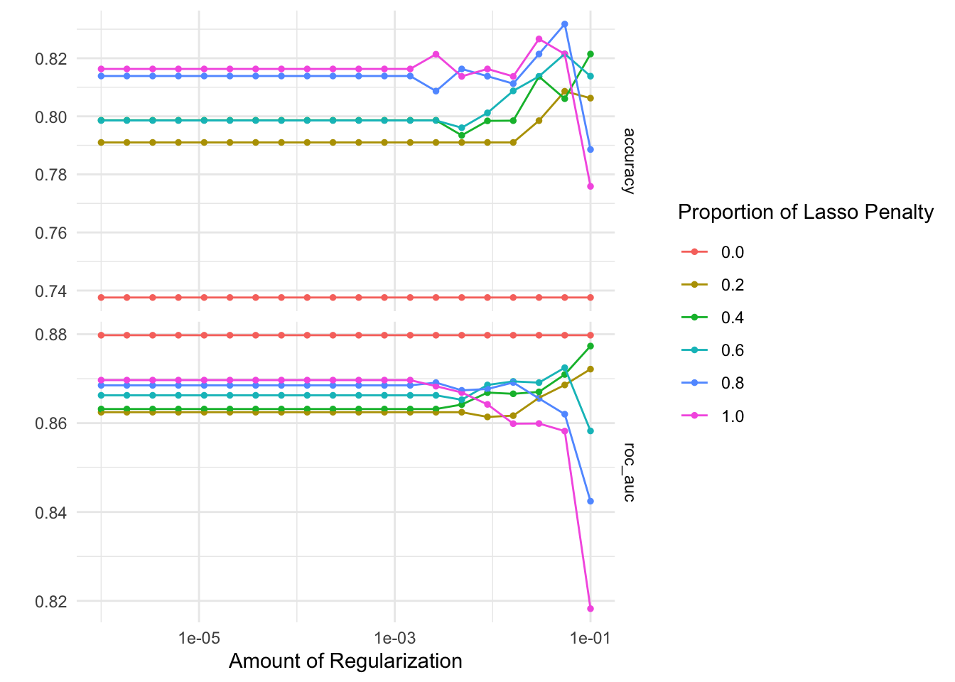
# identify the five best hyperparameter combinations
show_best(x = glmnet_tune, metric = "roc_auc")
## # A tibble: 5 × 8
##      penalty mixture .metric .estimator  mean     n std_err .config
##        <dbl>   <dbl> <chr>   <chr>      <dbl> <int>   <dbl> <chr>
## 1 0.000001         0 roc_auc binary     0.880    10  0.0180 Preprocessor1_Model…
## 2 0.00000183       0 roc_auc binary     0.880    10  0.0180 Preprocessor1_Model…
## 3 0.00000336       0 roc_auc binary     0.880    10  0.0180 Preprocessor1_Model…
## 4 0.00000616       0 roc_auc binary     0.880    10  0.0180 Preprocessor1_Model…
## 5 0.0000113        0 roc_auc binary     0.880    10  0.0180 Preprocessor1_Model…
Based on the ROC AUC, any penalty parameter with a mixture of 0 provides the optimal model performance. Though compared to the random forest model, the penalized regression approach consistently generates lower ROC AUC scores. This is likely because penalized regression models are a form of generalized linear models which assume linear, additive relationships between the predictors (i.e. n-grams) and the outcome of interest. Random forests are built from decision trees which are highly interactive and non-linear, so they allow for more flexible relationships between the predictors and outcome.
Fit the best model
- Select the hyperparameter combinations that achieve the highest ROC AUC
- Fit the penalized regression model using the best hyperparameters and the full training set. How well does the model perform on the test set?
Click for the solution
# select the best model's hyperparameters
glmnet_best <- select_best(glmnet_tune, metric = "roc_auc")

# fit a single model using the selected hyperparameters and the full training set
glmnet_final <- glmnet_workflow %>%
  finalize_workflow(parameters = glmnet_best) %>%
  last_fit(split = lyrics_split)
collect_metrics(glmnet_final)
## # A tibble: 2 × 4
##   .metric  .estimator .estimate .config
##   <chr>    <chr>          <dbl> <chr>
## 1 accuracy binary         0.756 Preprocessor1_Model1
## 2 roc_auc  binary         0.846 Preprocessor1_Model1
Not surprisingly the test set performance is slightly lower than the cross-validated metrics (ROC AUC of 0.85), however it still offers decent performance.
Variable importance
Beyond predictive power, we can analyze which n-grams contribute most strongly to the model’s predictions. Here we use the vip and vi() to calculate the importance score for each n-gram, then visualize them using a bar plot.
# extract parnsip model fit
glmnet_imp <- extract_fit_parsnip(glmnet_final) %>%
  # calculate variable importance for the specific penalty parameter used
  vi(lambda = glmnet_best$penalty)

# clean up the data frame for visualization
glmnet_imp %>%
  mutate(
    Sign = case_when(
      Sign == "POS" ~ "More likely from Beyoncé",
      Sign == "NEG" ~ "More likely from Taylor Swift"
    ),
    Importance = abs(Importance)
  ) %>%
  group_by(Sign) %>%
  # extract 20 most important n-grams for each artist
  slice_max(order_by = Importance, n = 20) %>%
  ggplot(mapping = aes(
    x = Importance,
    y = fct_reorder(Variable, Importance),
    fill = Sign
  )) +
  geom_col(show.legend = FALSE) +
  scale_x_continuous(expand = c(0, 0)) +
  scale_fill_brewer(type = "qual") +
  facet_wrap(facets = vars(Sign), scales = "free") +
  labs(
    y = NULL,
    title = "Variable importance for predicting the song artist",
    subtitle = "These features are the most important in predicting\nwhether a song is by Beyoncé or Taylor Swift"
  )
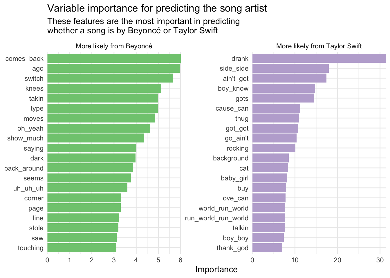
This helps provide facial validity for the model’s predictions. Not surprisingly, most of the n-grams relevant to Taylor Swift involve “love” and “baby”, whereas “girls girls” is likely generalized from “Run the World (Girls)”.
Acknowledgments
- Exercise inspired by the #TidyTuesday challenge on September 29, 2020.
Session Info
sessioninfo::session_info()
## ─ Session info ───────────────────────────────────────────────────────────────
##  setting  value
##  version  R version 4.2.1 (2022-06-23)
##  os       macOS Monterey 12.3
##  system   aarch64, darwin20
##  ui       X11
##  language (EN)
##  collate  en_US.UTF-8
##  ctype    en_US.UTF-8
##  tz       America/New_York
##  date     2022-11-16
##  pandoc   2.19.2 @ /Applications/RStudio.app/Contents/MacOS/quarto/bin/tools/ (via rmarkdown)
##
## ─ Packages ───────────────────────────────────────────────────────────────────
##  package       * version    date (UTC) lib source
##  assertthat      0.2.1      2019-03-21 [2] CRAN (R 4.2.0)
##  backports       1.4.1      2021-12-13 [2] CRAN (R 4.2.0)
##  bit             4.0.4      2020-08-04 [2] CRAN (R 4.2.0)
##  bit64           4.0.5      2020-08-30 [2] CRAN (R 4.2.0)
##  blogdown        1.10       2022-05-10 [2] CRAN (R 4.2.0)
##  bookdown        0.27       2022-06-14 [2] CRAN (R 4.2.0)
##  broom         * 1.0.0      2022-07-01 [2] CRAN (R 4.2.0)
##  bslib           0.4.0      2022-07-16 [2] CRAN (R 4.2.0)
##  cachem          1.0.6      2021-08-19 [2] CRAN (R 4.2.0)
##  cellranger      1.1.0      2016-07-27 [2] CRAN (R 4.2.0)
##  class           7.3-20     2022-01-16 [2] CRAN (R 4.2.1)
##  cli             3.4.1      2022-09-23 [1] CRAN (R 4.2.0)
##  codetools       0.2-18     2020-11-04 [2] CRAN (R 4.2.1)
##  colorspace      2.0-3      2022-02-21 [2] CRAN (R 4.2.0)
##  crayon          1.5.2      2022-09-29 [1] CRAN (R 4.2.0)
##  curl            4.3.3      2022-10-06 [1] CRAN (R 4.2.0)
##  DBI             1.1.3      2022-06-18 [2] CRAN (R 4.2.0)
##  dbplyr          2.2.1      2022-06-27 [2] CRAN (R 4.2.0)
##  dials         * 1.0.0      2022-06-14 [2] CRAN (R 4.2.0)
##  DiceDesign      1.9        2021-02-13 [2] CRAN (R 4.2.0)
##  digest          0.6.29     2021-12-01 [2] CRAN (R 4.2.0)
##  dplyr         * 1.0.10     2022-09-01 [1] CRAN (R 4.2.0)
##  ellipsis        0.3.2      2021-04-29 [2] CRAN (R 4.2.0)
##  evaluate        0.18       2022-11-07 [1] CRAN (R 4.2.0)
##  fansi           1.0.3      2022-03-24 [2] CRAN (R 4.2.0)
##  farver          2.1.1      2022-07-06 [2] CRAN (R 4.2.0)
##  fastmap         1.1.0      2021-01-25 [2] CRAN (R 4.2.0)
##  forcats       * 0.5.2      2022-08-19 [1] CRAN (R 4.2.0)
##  foreach         1.5.2      2022-02-02 [2] CRAN (R 4.2.0)
##  fs              1.5.2      2021-12-08 [2] CRAN (R 4.2.0)
##  furrr           0.3.0      2022-05-04 [2] CRAN (R 4.2.0)
##  future          1.27.0     2022-07-22 [2] CRAN (R 4.2.0)
##  future.apply    1.9.0      2022-04-25 [2] CRAN (R 4.2.0)
##  gargle          1.2.0      2021-07-02 [2] CRAN (R 4.2.0)
##  generics        0.1.3      2022-07-05 [2] CRAN (R 4.2.0)
##  ggplot2       * 3.3.6      2022-05-03 [2] CRAN (R 4.2.0)
##  glmnet        * 4.1-4      2022-04-15 [2] CRAN (R 4.2.0)
##  globals         0.16.0     2022-08-05 [2] CRAN (R 4.2.0)
##  glue            1.6.2      2022-02-24 [2] CRAN (R 4.2.0)
##  googledrive     2.0.0      2021-07-08 [2] CRAN (R 4.2.0)
##  googlesheets4   1.0.0      2021-07-21 [2] CRAN (R 4.2.0)
##  gower           1.0.0      2022-02-03 [2] CRAN (R 4.2.0)
##  GPfit           1.0-8      2019-02-08 [2] CRAN (R 4.2.0)
##  gridExtra       2.3        2017-09-09 [2] CRAN (R 4.2.0)
##  gtable          0.3.1      2022-09-01 [1] CRAN (R 4.2.0)
##  hardhat         1.2.0      2022-06-30 [2] CRAN (R 4.2.0)
##  haven           2.5.1      2022-08-22 [1] CRAN (R 4.2.0)
##  here          * 1.0.1      2020-12-13 [2] CRAN (R 4.2.0)
##  highr           0.9        2021-04-16 [2] CRAN (R 4.2.0)
##  hms             1.1.2      2022-08-19 [1] CRAN (R 4.2.0)
##  htmltools       0.5.3      2022-07-18 [2] CRAN (R 4.2.0)
##  httr            1.4.3      2022-05-04 [2] CRAN (R 4.2.0)
##  infer         * 1.0.2      2022-06-10 [2] CRAN (R 4.2.0)
##  ipred           0.9-13     2022-06-02 [2] CRAN (R 4.2.0)
##  iterators       1.0.14     2022-02-05 [2] CRAN (R 4.2.0)
##  jquerylib       0.1.4      2021-04-26 [2] CRAN (R 4.2.0)
##  jsonlite        1.8.0      2022-02-22 [2] CRAN (R 4.2.0)
##  knitr           1.40       2022-08-24 [1] CRAN (R 4.2.0)
##  labeling        0.4.2      2020-10-20 [2] CRAN (R 4.2.0)
##  lattice         0.20-45    2021-09-22 [2] CRAN (R 4.2.1)
##  lava            1.6.10     2021-09-02 [2] CRAN (R 4.2.0)
##  lhs             1.1.5      2022-03-22 [2] CRAN (R 4.2.0)
##  lifecycle       1.0.3      2022-10-07 [1] CRAN (R 4.2.0)
##  listenv         0.8.0      2019-12-05 [2] CRAN (R 4.2.0)
##  lubridate       1.8.0      2021-10-07 [2] CRAN (R 4.2.0)
##  magrittr        2.0.3      2022-03-30 [2] CRAN (R 4.2.0)
##  MASS            7.3-58.1   2022-08-03 [2] CRAN (R 4.2.0)
##  Matrix        * 1.4-1      2022-03-23 [2] CRAN (R 4.2.1)
##  modeldata     * 1.0.0      2022-07-01 [2] CRAN (R 4.2.0)
##  modelr          0.1.8      2020-05-19 [2] CRAN (R 4.2.0)
##  munsell         0.5.0      2018-06-12 [2] CRAN (R 4.2.0)
##  nnet            7.3-17     2022-01-16 [2] CRAN (R 4.2.1)
##  parallelly      1.32.1     2022-07-21 [2] CRAN (R 4.2.0)
##  parsnip       * 1.0.0      2022-06-16 [2] CRAN (R 4.2.0)
##  pillar          1.8.1      2022-08-19 [1] CRAN (R 4.2.0)
##  pkgconfig       2.0.3      2019-09-22 [2] CRAN (R 4.2.0)
##  prodlim         2019.11.13 2019-11-17 [2] CRAN (R 4.2.0)
##  purrr         * 0.3.5      2022-10-06 [1] CRAN (R 4.2.0)
##  R6              2.5.1      2021-08-19 [2] CRAN (R 4.2.0)
##  ranger        * 0.14.1     2022-06-18 [2] CRAN (R 4.2.0)
##  RColorBrewer    1.1-3      2022-04-03 [2] CRAN (R 4.2.0)
##  Rcpp            1.0.9      2022-07-08 [2] CRAN (R 4.2.0)
##  readr         * 2.1.3      2022-10-01 [1] CRAN (R 4.2.0)
##  readxl          1.4.0      2022-03-28 [2] CRAN (R 4.2.0)
##  recipes       * 1.0.1      2022-07-07 [2] CRAN (R 4.2.0)
##  reprex          2.0.2      2022-08-17 [1] CRAN (R 4.2.0)
##  rlang         * 1.0.6      2022-09-24 [1] CRAN (R 4.2.0)
##  rmarkdown       2.14       2022-04-25 [2] CRAN (R 4.2.0)
##  ROSE            0.0-4      2021-06-14 [2] CRAN (R 4.2.0)
##  rpart           4.1.16     2022-01-24 [2] CRAN (R 4.2.1)
##  rprojroot       2.0.3      2022-04-02 [2] CRAN (R 4.2.0)
##  rsample       * 1.1.0      2022-08-08 [2] CRAN (R 4.2.1)
##  rstudioapi      0.13       2020-11-12 [2] CRAN (R 4.2.0)
##  rvest           1.0.2      2021-10-16 [2] CRAN (R 4.2.0)
##  sass            0.4.2      2022-07-16 [2] CRAN (R 4.2.0)
##  scales        * 1.2.1      2022-08-20 [1] CRAN (R 4.2.0)
##  sessioninfo     1.2.2      2021-12-06 [2] CRAN (R 4.2.0)
##  shape           1.4.6      2021-05-19 [2] CRAN (R 4.2.0)
##  SnowballC       0.7.0      2020-04-01 [2] CRAN (R 4.2.0)
##  stopwords     * 2.3        2021-10-28 [2] CRAN (R 4.2.0)
##  stringi         1.7.8      2022-07-11 [2] CRAN (R 4.2.0)
##  stringr       * 1.4.0      2019-02-10 [2] CRAN (R 4.2.0)
##  survival        3.3-1      2022-03-03 [2] CRAN (R 4.2.1)
##  textrecipes   * 1.0.0      2022-07-02 [2] CRAN (R 4.2.0)
##  themis        * 1.0.0      2022-07-02 [2] CRAN (R 4.2.0)
##  tibble        * 3.1.8      2022-07-22 [2] CRAN (R 4.2.0)
##  tidymodels    * 1.0.0      2022-07-13 [2] CRAN (R 4.2.0)
##  tidyr         * 1.2.0      2022-02-01 [2] CRAN (R 4.2.0)
##  tidyselect      1.2.0      2022-10-10 [1] CRAN (R 4.2.0)
##  tidyverse     * 1.3.2      2022-07-18 [2] CRAN (R 4.2.0)
##  timeDate        4021.104   2022-07-19 [2] CRAN (R 4.2.0)
##  tokenizers      0.2.1      2018-03-29 [2] CRAN (R 4.2.0)
##  tune          * 1.0.0      2022-07-07 [2] CRAN (R 4.2.0)
##  tzdb            0.3.0      2022-03-28 [2] CRAN (R 4.2.0)
##  utf8            1.2.2      2021-07-24 [2] CRAN (R 4.2.0)
##  vctrs         * 0.5.0      2022-10-22 [1] CRAN (R 4.2.0)
##  vip           * 0.3.2      2020-12-17 [2] CRAN (R 4.2.0)
##  vroom           1.6.0      2022-09-30 [1] CRAN (R 4.2.0)
##  withr           2.5.0      2022-03-03 [2] CRAN (R 4.2.0)
##  workflows     * 1.0.0      2022-07-05 [2] CRAN (R 4.2.0)
##  workflowsets  * 1.0.0      2022-07-12 [2] CRAN (R 4.2.0)
##  xfun            0.34       2022-10-18 [1] CRAN (R 4.2.0)
##  xml2            1.3.3      2021-11-30 [2] CRAN (R 4.2.0)
##  yaml            2.3.5      2022-02-21 [2] CRAN (R 4.2.0)
##  yardstick     * 1.0.0      2022-06-06 [2] CRAN (R 4.2.0)
##
##  [1] /Users/soltoffbc/Library/R/arm64/4.2/library
##  [2] /Library/Frameworks/R.framework/Versions/4.2-arm64/Resources/library
##
## ──────────────────────────────────────────────────────────────────────────────
Importantly, the Beyoncé lyrics are originally stored as one row per line per song whereas we need them stored as one row per song for modeling purposes. ↩︎