Practicing sentiment analysis with Harry Potter
library(tidyverse)
library(tidytext)
library(harrypotter)

set.seed(1234)
theme_set(theme_minimal())
Run the code below in your console to download this exercise as a set of R scripts.
usethis::use_course("cis-ds/text-analysis-fundamentals-and-sentiment-analysis")
Load Harry Potter text
Run the following code to download the harrypotter package:
remotes::install_github("bradleyboehmke/harrypotter")
Note that there is a different package available on CRAN also called harrypotter. This is an entirely different package. If you just run install.packages("harrypotter"), you will get an error.
library(harrypotter)

# names of each book
hp_books <- c(
  "philosophers_stone", "chamber_of_secrets",
  "prisoner_of_azkaban", "goblet_of_fire",
  "order_of_the_phoenix", "half_blood_prince",
  "deathly_hallows"
)

# combine books into a list
hp_words <- list(
  philosophers_stone,
  chamber_of_secrets,
  prisoner_of_azkaban,
  goblet_of_fire,
  order_of_the_phoenix,
  half_blood_prince,
  deathly_hallows
) %>%
  # name each list element
  set_names(hp_books) %>%
  # convert each book to a data frame and merge into a single data frame
  map_df(as_tibble, .id = "book") %>%
  # convert book to a factor
  mutate(book = factor(book, levels = hp_books)) %>%
  # remove empty chapters
  drop_na(value) %>%
  # create a chapter id column
  group_by(book) %>%
  mutate(chapter = row_number(book)) %>%
  ungroup() %>%
  # tokenize the data frame
  unnest_tokens(word, value)

hp_words
## # A tibble: 1,089,386 × 3
##    book               chapter word
##    <fct>                <int> <chr>
##  1 philosophers_stone       1 the
##  2 philosophers_stone       1 boy
##  3 philosophers_stone       1 who
##  4 philosophers_stone       1 lived
##  5 philosophers_stone       1 mr
##  6 philosophers_stone       1 and
##  7 philosophers_stone       1 mrs
##  8 philosophers_stone       1 dursley
##  9 philosophers_stone       1 of
## 10 philosophers_stone       1 number
## # … with 1,089,376 more rows
## # ℹ Use `print(n = ...)` to see more rows
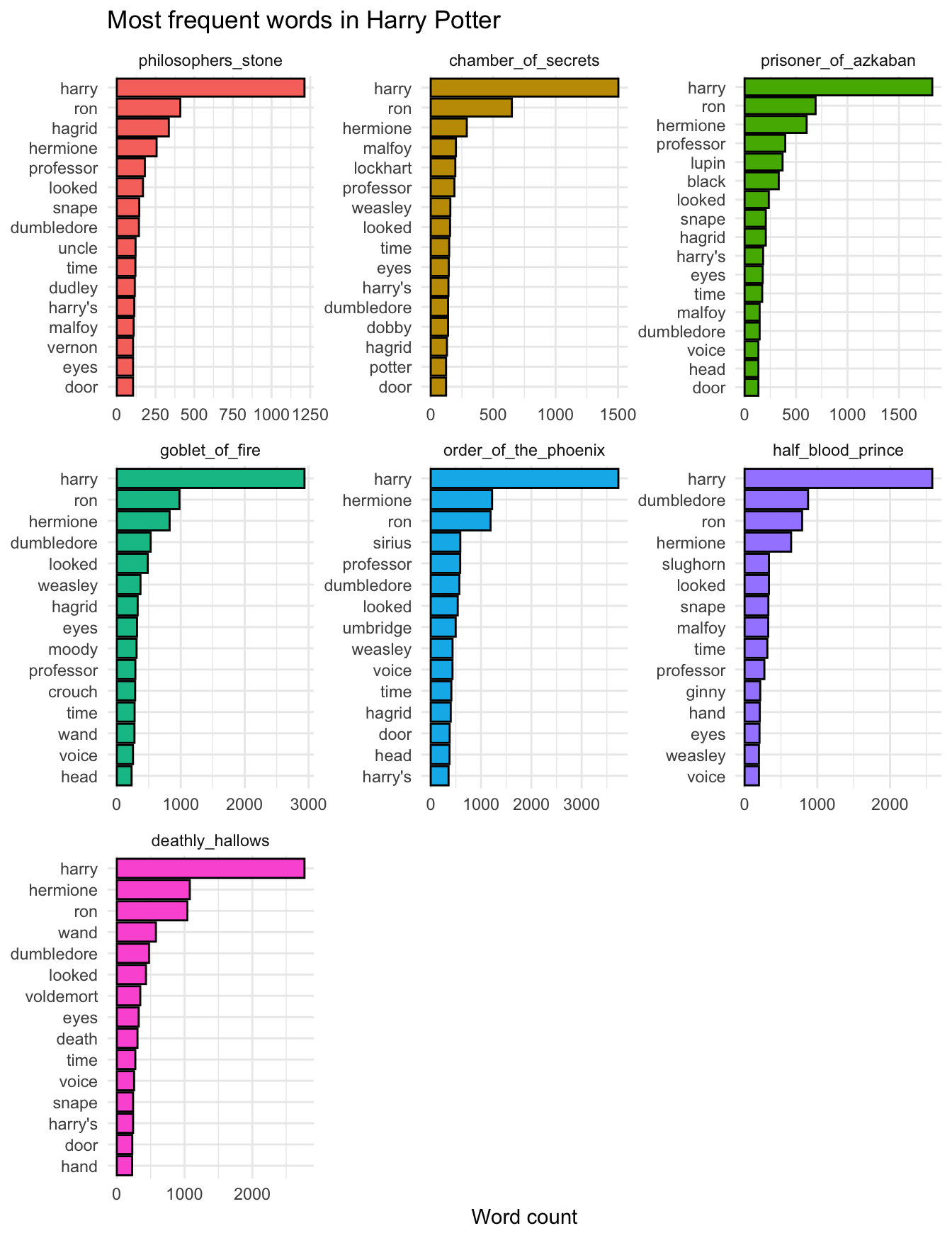
Most frequent words, by book
Remove stop words.
hp_words %>%
  # delete stopwords
  anti_join(stop_words) %>%
  # summarize count per word per book
  count(book, word) %>%
  # get top 15 words per book
  group_by(book) %>%
  slice_max(order_by = n, n = 15) %>%
  mutate(word = reorder_within(word, n, book)) %>%
  # create barplot
  ggplot(aes(x = word, y = n, fill = book)) +
  geom_col(color = "black") +
  scale_x_reordered() +
  labs(
    title = "Most frequent words in Harry Potter",
    x = NULL,
    y = "Word count"
  ) +
  facet_wrap(facets = vars(book), scales = "free") +
  coord_flip() +
  theme(legend.position = "none")
## Joining, by = "word"
Estimate sentiment
Generate data frame with sentiment derived from the Bing dictionary
Click for the solution
(hp_bing <- hp_words %>%
  inner_join(get_sentiments("bing")))
## Joining, by = "word"
## # A tibble: 65,094 × 4
##    book               chapter word       sentiment
##    <fct>                <int> <chr>      <chr>
##  1 philosophers_stone       1 proud      positive
##  2 philosophers_stone       1 perfectly  positive
##  3 philosophers_stone       1 thank      positive
##  4 philosophers_stone       1 strange    negative
##  5 philosophers_stone       1 mysterious negative
##  6 philosophers_stone       1 nonsense   negative
##  7 philosophers_stone       1 useful     positive
##  8 philosophers_stone       1 finer      positive
##  9 philosophers_stone       1 greatest   positive
## 10 philosophers_stone       1 fear       negative
## # … with 65,084 more rows
## # ℹ Use `print(n = ...)` to see more rows
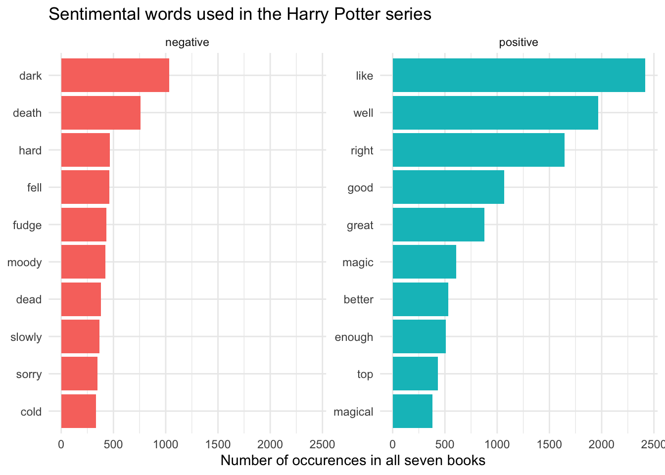
Visualize the most frequent positive/negative words in the entire series using the Bing dictionary, and then separately for each book
reorder_within() and scale_x_reordered() functions for sorting bar charts within each facet.Click for the solution
# all series
hp_bing %>%
  # generate frequency count for each word and sentiment
  group_by(sentiment) %>%
  count(word) %>%
  # extract 10 most frequent pos/neg words
  group_by(sentiment) %>%
  slice_max(order_by = n, n = 10) %>%
  # prep data for sorting each word independently by facet
  mutate(word = reorder_within(word, n, sentiment)) %>%
  # generate the bar plot
  ggplot(aes(word, n, fill = sentiment)) +
  geom_col(show.legend = FALSE) +
  # used with reorder_within() to label the axis tick marks
  scale_x_reordered() +
  facet_wrap(facets = vars(sentiment), scales = "free_y") +
  labs(
    title = "Sentimental words used in the Harry Potter series",
    x = NULL,
    y = "Number of occurences in all seven books"
  ) +
  coord_flip()
# per book
hp_pos_neg_book <- hp_bing %>%
# generate frequency count for each book, word, and sentiment
group_by(book, sentiment) %>%
count(word) %>%
# extract 10 most frequent pos/neg words per book
group_by(book, sentiment) %>%
slice_max(order_by = n, n = 10)
## positive words
hp_pos_neg_book %>%
filter(sentiment == "positive") %>%
mutate(word = reorder_within(word, n, book)) %>%
ggplot(aes(word, n)) +
geom_col(show.legend = FALSE) +
scale_x_reordered() +
facet_wrap(facets = vars(book), scales = "free_y") +
labs(
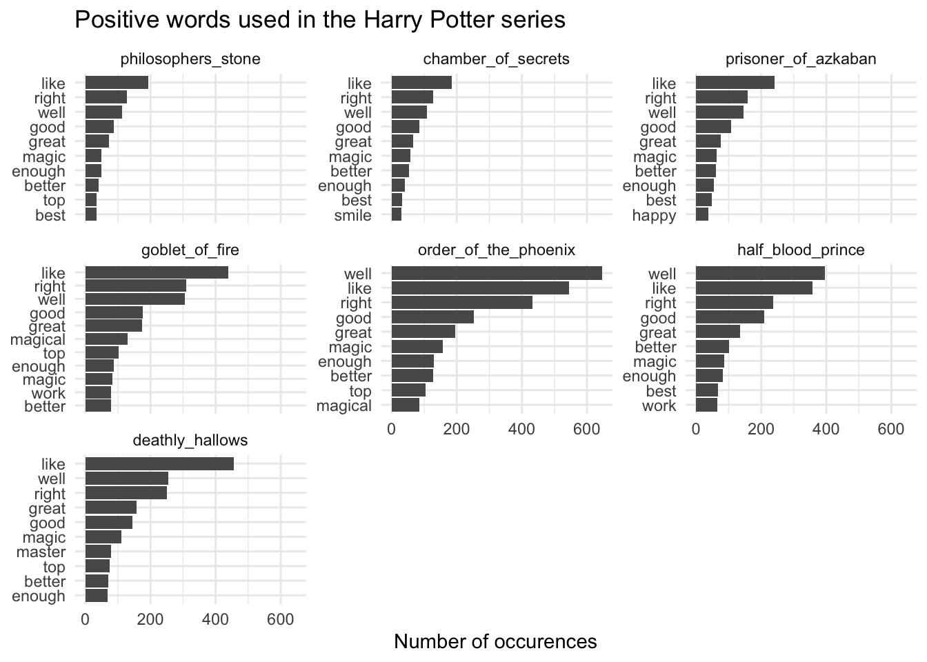
title = "Positive words used in the Harry Potter series",
x = NULL,
y = "Number of occurences"
) +
coord_flip()
## negative words
hp_pos_neg_book %>%
filter(sentiment == "negative") %>%
mutate(word = reorder_within(word, n, book)) %>%
ggplot(aes(word, n)) +
geom_col(show.legend = FALSE) +
scale_x_reordered() +
facet_wrap(facets = vars(book), scales = "free_y") +
labs(
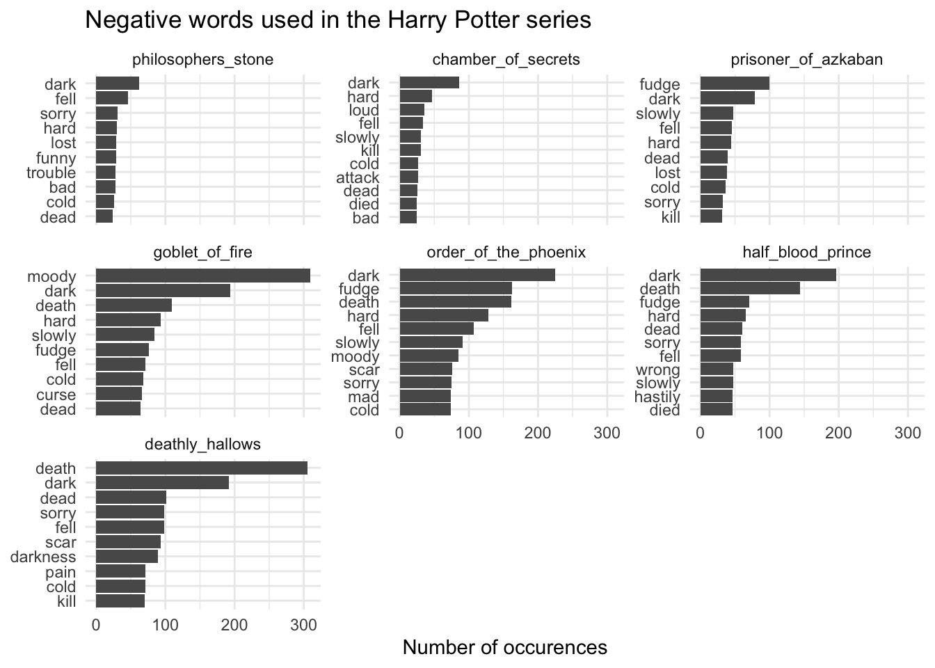
title = "Negative words used in the Harry Potter series",
x = NULL,
y = "Number of occurences"
) +
coord_flip()
Generate data frame with sentiment derived from the AFINN dictionary
Click for the solution
(hp_afinn <- hp_words %>%
  inner_join(get_sentiments("afinn")) %>%
  group_by(book, chapter))
## Joining, by = "word"
## # A tibble: 56,311 × 4
## # Groups:   book, chapter [200]
##    book               chapter word      value
##    <fct>                <int> <chr>     <dbl>
##  1 philosophers_stone       1 proud         2
##  2 philosophers_stone       1 perfectly     3
##  3 philosophers_stone       1 thank         2
##  4 philosophers_stone       1 strange      -1
##  5 philosophers_stone       1 nonsense     -2
##  6 philosophers_stone       1 big           1
##  7 philosophers_stone       1 useful        2
##  8 philosophers_stone       1 no           -1
##  9 philosophers_stone       1 greatest      3
## 10 philosophers_stone       1 fear         -2
## # … with 56,301 more rows
## # ℹ Use `print(n = ...)` to see more rows
Visualize which words in the AFINN sentiment dictionary appear most frequently
Sometimes words which are defined in a general sentiment dictionary can be outliers in specific contexts. That is, an author may use a word without intending to convey a specific sentiment but the dictionary defines it in a certain way.
We can use a wordcloud as a quick check to see if there are any outliers in the context of Harry Potter, constructed using ggwordcloud:
library(ggwordcloud)

set.seed(123) # ensure reproducibility of the wordcloud
hp_afinn %>%
  # count word frequency across books
  ungroup() %>%
  count(word) %>%
  # keep only top 100 words for wordcloud
  slice_max(order_by = n, n = 100) %>%
  mutate(angle = 90 * sample(c(0, 1), n(), replace = TRUE, prob = c(70, 30))) %>%
  ggplot(aes(label = word, size = n, angle = angle)) +
  geom_text_wordcloud(rm_outside = TRUE) +
  scale_size_area(max_size = 15) +
  ggtitle("Most frequent tokens in Harry Potter") +
  theme_minimal()
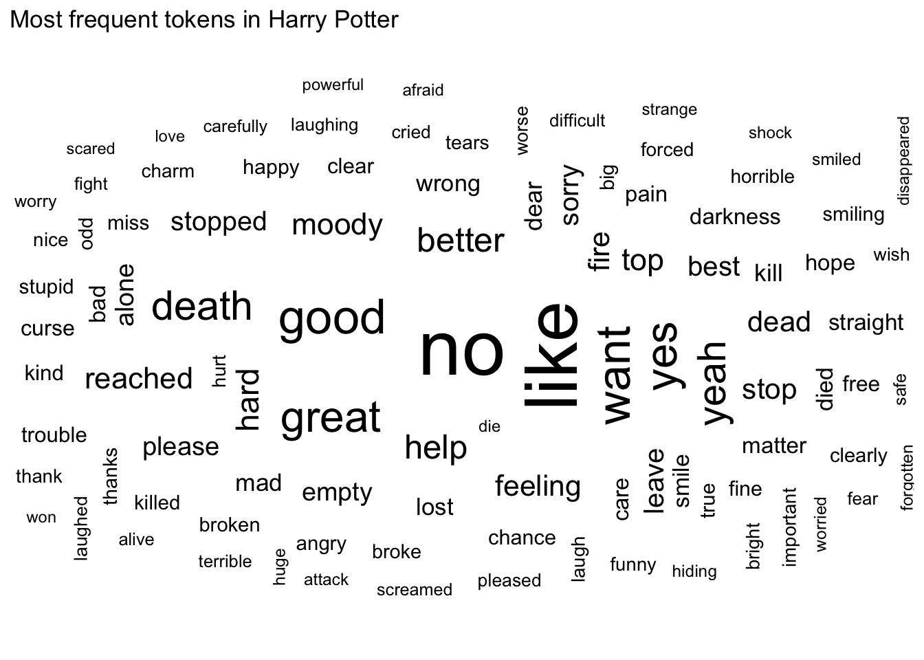
As we can see, “moody” appears quite frequently in the books. In the vast majority of appearances, “moody” is used to refer to the character Alastor “Mad-Eye” Moody and is not meant to convey a specific sentiment.
hp_afinn %>%
  filter(word == "moody")
## # A tibble: 422 × 4
## # Groups:   book, chapter [48]
##    book               chapter word  value
##    <fct>                <int> <chr> <dbl>
##  1 chamber_of_secrets      13 moody    -1
##  2 goblet_of_fire          11 moody    -1
##  3 goblet_of_fire          11 moody    -1
##  4 goblet_of_fire          11 moody    -1
##  5 goblet_of_fire          12 moody    -1
##  6 goblet_of_fire          12 moody    -1
##  7 goblet_of_fire          12 moody    -1
##  8 goblet_of_fire          12 moody    -1
##  9 goblet_of_fire          12 moody    -1
## 10 goblet_of_fire          12 moody    -1
## # … with 412 more rows
## # ℹ Use `print(n = ...)` to see more rows
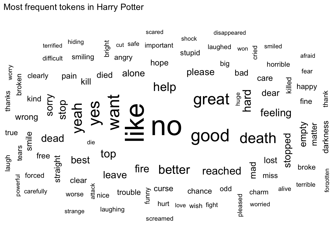
It would be best to remove this word from further sentiment analysis, treating it as if it were another stop word.
hp_afinn <- hp_afinn %>%
  filter(word != "moody")

# wordcloud without harry
set.seed(123) # ensure reproducibility of the wordcloud
hp_afinn %>%
  # count word frequency across books
  ungroup() %>%
  count(word) %>%
  # keep only top 100 words for wordcloud
  slice_max(order_by = n, n = 100) %>%
  mutate(angle = 90 * sample(c(0, 1), n(), replace = TRUE, prob = c(70, 30))) %>%
  ggplot(aes(label = word, size = n, angle = angle)) +
  geom_text_wordcloud(rm_outside = TRUE) +
  scale_size_area(max_size = 15) +
  ggtitle("Most frequent tokens in Harry Potter") +
  theme_minimal()
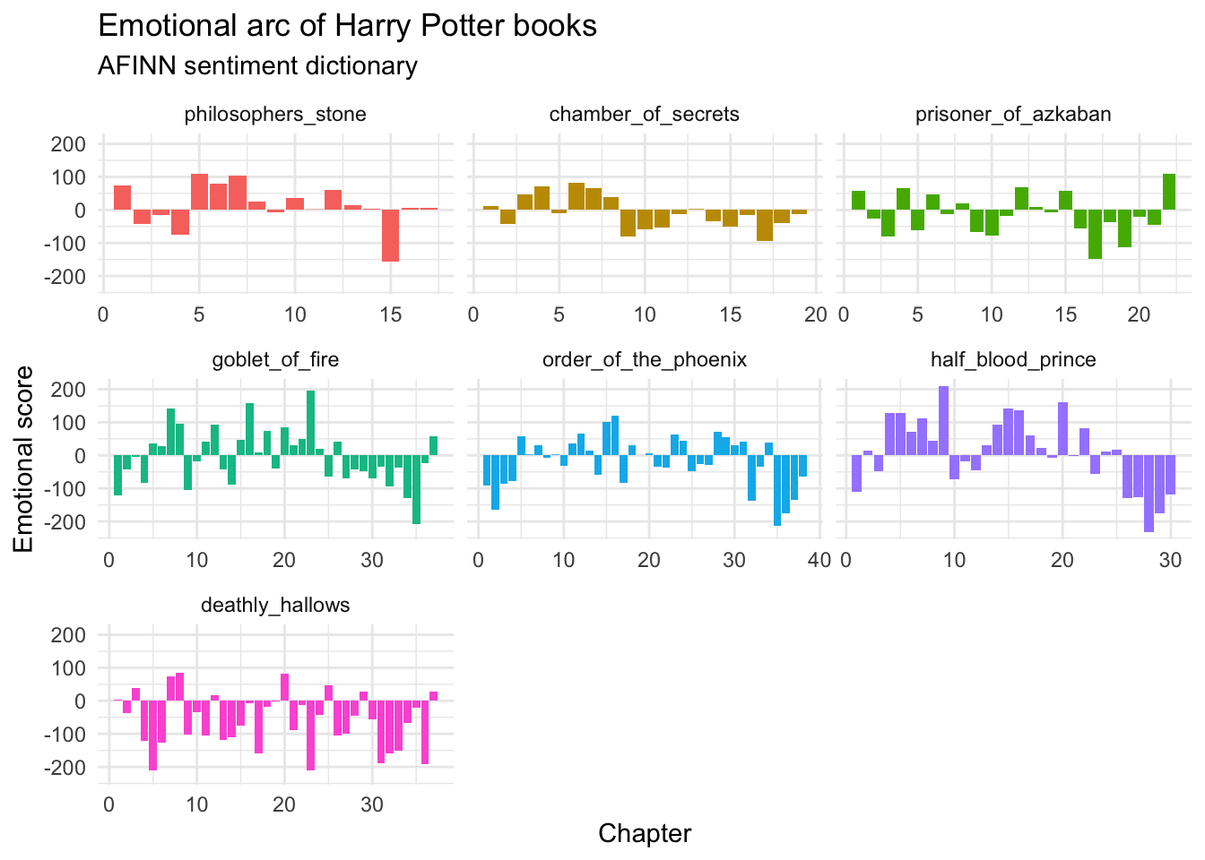
Visualize the positive/negative sentiment for each book over time using the AFINN dictionary
Click for the solution
hp_words %>%
  inner_join(get_sentiments("afinn")) %>%
  group_by(book, chapter) %>%
  summarize(value = sum(value)) %>%
  ggplot(mapping = aes(x = chapter, y = value, fill = book)) +
  geom_col() +
  facet_wrap(facets = vars(book), scales = "free_x") +
  labs(
    title = "Emotional arc of Harry Potter books",
    subtitle = "AFINN sentiment dictionary",
    x = "Chapter",
    y = "Emotional score"
  ) +
  theme(legend.position = "none")
## Joining, by = "word"
## `summarise()` has grouped output by 'book'. You can override using the
## `.groups` argument.
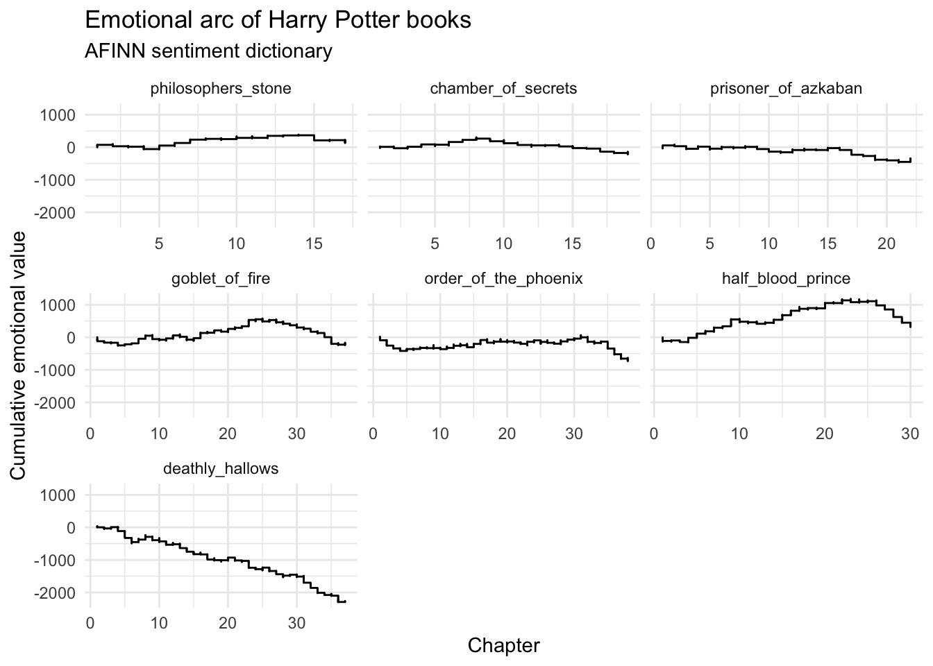
# cumulative value
hp_words %>%
  inner_join(get_sentiments("afinn")) %>%
  group_by(book) %>%
  mutate(cumvalue = cumsum(value)) %>%
  ggplot(mapping = aes(x = chapter, y = cumvalue, fill = book)) +
  geom_step() +
  facet_wrap(facets = vars(book), scales = "free_x") +
  labs(
    title = "Emotional arc of Harry Potter books",
    subtitle = "AFINN sentiment dictionary",
    x = "Chapter",
    y = "Cumulative emotional value"
  )
## Joining, by = "word"
Acknowledgments
- This page is derived in part from Harry Plotter: Celebrating the 20 year anniversary with
tidytextand thetidyversein R and licensed under a Creative Commons Attribution-ShareAlike 4.0 International License.
Session Info
sessioninfo::session_info()
## ─ Session info ───────────────────────────────────────────────────────────────
##  setting  value
##  version  R version 4.2.1 (2022-06-23)
##  os       macOS Monterey 12.3
##  system   aarch64, darwin20
##  ui       X11
##  language (EN)
##  collate  en_US.UTF-8
##  ctype    en_US.UTF-8
##  tz       America/New_York
##  date     2022-08-22
##  pandoc   2.18 @ /Applications/RStudio.app/Contents/MacOS/quarto/bin/tools/ (via rmarkdown)
##
## ─ Packages ───────────────────────────────────────────────────────────────────
##  package       * version    date (UTC) lib source
##  assertthat      0.2.1      2019-03-21 [2] CRAN (R 4.2.0)
##  backports       1.4.1      2021-12-13 [2] CRAN (R 4.2.0)
##  blogdown        1.10       2022-05-10 [2] CRAN (R 4.2.0)
##  bookdown        0.27       2022-06-14 [2] CRAN (R 4.2.0)
##  broom           1.0.0      2022-07-01 [2] CRAN (R 4.2.0)
##  bslib           0.4.0      2022-07-16 [2] CRAN (R 4.2.0)
##  cachem          1.0.6      2021-08-19 [2] CRAN (R 4.2.0)
##  cellranger      1.1.0      2016-07-27 [2] CRAN (R 4.2.0)
##  cli             3.3.0      2022-04-25 [2] CRAN (R 4.2.0)
##  colorspace      2.0-3      2022-02-21 [2] CRAN (R 4.2.0)
##  crayon          1.5.1      2022-03-26 [2] CRAN (R 4.2.0)
##  DBI             1.1.3      2022-06-18 [2] CRAN (R 4.2.0)
##  dbplyr          2.2.1      2022-06-27 [2] CRAN (R 4.2.0)
##  digest          0.6.29     2021-12-01 [2] CRAN (R 4.2.0)
##  dplyr         * 1.0.9      2022-04-28 [2] CRAN (R 4.2.0)
##  ellipsis        0.3.2      2021-04-29 [2] CRAN (R 4.2.0)
##  evaluate        0.16       2022-08-09 [1] CRAN (R 4.2.1)
##  fansi           1.0.3      2022-03-24 [2] CRAN (R 4.2.0)
##  fastmap         1.1.0      2021-01-25 [2] CRAN (R 4.2.0)
##  forcats       * 0.5.1      2021-01-27 [2] CRAN (R 4.2.0)
##  fs              1.5.2      2021-12-08 [2] CRAN (R 4.2.0)
##  gargle          1.2.0      2021-07-02 [2] CRAN (R 4.2.0)
##  generics        0.1.3      2022-07-05 [2] CRAN (R 4.2.0)
##  ggplot2       * 3.3.6      2022-05-03 [2] CRAN (R 4.2.0)
##  glue            1.6.2      2022-02-24 [2] CRAN (R 4.2.0)
##  googledrive     2.0.0      2021-07-08 [2] CRAN (R 4.2.0)
##  googlesheets4   1.0.0      2021-07-21 [2] CRAN (R 4.2.0)
##  gtable          0.3.0      2019-03-25 [2] CRAN (R 4.2.0)
##  harrypotter   * 0.1.0      2022-08-22 [1] Github (bradleyboehmke/harrypotter@51f7146)
##  haven           2.5.0      2022-04-15 [2] CRAN (R 4.2.0)
##  here            1.0.1      2020-12-13 [2] CRAN (R 4.2.0)
##  hms             1.1.1      2021-09-26 [2] CRAN (R 4.2.0)
##  htmltools       0.5.3      2022-07-18 [2] CRAN (R 4.2.0)
##  httr            1.4.3      2022-05-04 [2] CRAN (R 4.2.0)
##  janeaustenr     0.1.5      2017-06-10 [2] CRAN (R 4.2.0)
##  jquerylib       0.1.4      2021-04-26 [2] CRAN (R 4.2.0)
##  jsonlite        1.8.0      2022-02-22 [2] CRAN (R 4.2.0)
##  knitr           1.39       2022-04-26 [2] CRAN (R 4.2.0)
##  lattice         0.20-45    2021-09-22 [2] CRAN (R 4.2.1)
##  lifecycle       1.0.1      2021-09-24 [2] CRAN (R 4.2.0)
##  lubridate       1.8.0      2021-10-07 [2] CRAN (R 4.2.0)
##  magrittr        2.0.3      2022-03-30 [2] CRAN (R 4.2.0)
##  Matrix          1.4-1      2022-03-23 [2] CRAN (R 4.2.1)
##  modelr          0.1.8      2020-05-19 [2] CRAN (R 4.2.0)
##  munsell         0.5.0      2018-06-12 [2] CRAN (R 4.2.0)
##  pillar          1.8.0      2022-07-18 [2] CRAN (R 4.2.0)
##  pkgconfig       2.0.3      2019-09-22 [2] CRAN (R 4.2.0)
##  purrr         * 0.3.4      2020-04-17 [2] CRAN (R 4.2.0)
##  R6              2.5.1      2021-08-19 [2] CRAN (R 4.2.0)
##  Rcpp            1.0.9      2022-07-08 [2] CRAN (R 4.2.0)
##  readr         * 2.1.2      2022-01-30 [2] CRAN (R 4.2.0)
##  readxl          1.4.0      2022-03-28 [2] CRAN (R 4.2.0)
##  reprex          2.0.1.9000 2022-08-10 [1] Github (tidyverse/reprex@6d3ad07)
##  rlang           1.0.4      2022-07-12 [2] CRAN (R 4.2.0)
##  rmarkdown       2.14       2022-04-25 [2] CRAN (R 4.2.0)
##  rprojroot       2.0.3      2022-04-02 [2] CRAN (R 4.2.0)
##  rstudioapi      0.13       2020-11-12 [2] CRAN (R 4.2.0)
##  rvest           1.0.2      2021-10-16 [2] CRAN (R 4.2.0)
##  sass            0.4.2      2022-07-16 [2] CRAN (R 4.2.0)
##  scales          1.2.0      2022-04-13 [2] CRAN (R 4.2.0)
##  sessioninfo     1.2.2      2021-12-06 [2] CRAN (R 4.2.0)
##  SnowballC       0.7.0      2020-04-01 [2] CRAN (R 4.2.0)
##  stringi         1.7.8      2022-07-11 [2] CRAN (R 4.2.0)
##  stringr       * 1.4.0      2019-02-10 [2] CRAN (R 4.2.0)
##  tibble        * 3.1.8      2022-07-22 [2] CRAN (R 4.2.0)
##  tidyr         * 1.2.0      2022-02-01 [2] CRAN (R 4.2.0)
##  tidyselect      1.1.2      2022-02-21 [2] CRAN (R 4.2.0)
##  tidytext      * 0.3.3      2022-05-09 [2] CRAN (R 4.2.0)
##  tidyverse     * 1.3.2      2022-07-18 [2] CRAN (R 4.2.0)
##  tokenizers      0.2.1      2018-03-29 [2] CRAN (R 4.2.0)
##  tzdb            0.3.0      2022-03-28 [2] CRAN (R 4.2.0)
##  utf8            1.2.2      2021-07-24 [2] CRAN (R 4.2.0)
##  vctrs           0.4.1      2022-04-13 [2] CRAN (R 4.2.0)
##  withr           2.5.0      2022-03-03 [2] CRAN (R 4.2.0)
##  xfun            0.31       2022-05-10 [1] CRAN (R 4.2.0)
##  xml2            1.3.3      2021-11-30 [2] CRAN (R 4.2.0)
##  yaml            2.3.5      2022-02-21 [2] CRAN (R 4.2.0)
##
##  [1] /Users/soltoffbc/Library/R/arm64/4.2/library
##  [2] /Library/Frameworks/R.framework/Versions/4.2-arm64/Resources/library
##
## ──────────────────────────────────────────────────────────────────────────────