Practicing tidytext with Hamilton
library(tidyverse)
library(tidytext)
library(ggtext)
library(here)

set.seed(123)
theme_set(theme_minimal())
About seven months ago, my wife and I became addicted to Hamilton.
I admit, we were quite late to the party. I promise we did like it, but I wanted to wait and see the musical in-person before listening to the soundtrack. Alas, having three small children limits your free time to go out to the theater for an entire evening. So I finally caved and started listening to the soundtrack on Spotify. And it’s amazing! My son’s favorite song (he’s four BTW) is My Shot.
One of the nice things about the musical is that it is sung-through, so the lyrics contain essentially all of the dialogue. This provides an interesting opportunity to use the tidytext package to analyze the lyrics. Here, I use the geniusr package to obtain the complete lyrics from Genius.1
hamilton <- read_csv(file = here("static", "data", "hamilton.csv")) %>%
  mutate(song_name = parse_factor(song_name))
## Rows: 3532 Columns: 5
## ── Column specification ────────────────────────────────────────────────────────
## Delimiter: ","
## chr (3): song_name, line, speaker
## dbl (2): song_number, line_num
##
## ℹ Use `spec()` to retrieve the full column specification for this data.
## ℹ Specify the column types or set `show_col_types = FALSE` to quiet this message.
glimpse(hamilton)
## Rows: 3,532
## Columns: 5
## $ song_number <dbl> 1, 1, 1, 1, 1, 1, 1, 1, 1, 1, 1, 1, 1, 1, 1, 1, 1, 1, 1, 1…
## $ song_name   <fct> "Alexander Hamilton", "Alexander Hamilton", "Alexander Ham…
## $ line_num    <dbl> 1, 2, 3, 4, 5, 6, 7, 8, 9, 10, 11, 12, 13, 14, 15, 16, 17,…
## $ line        <chr> "How does a bastard, orphan, son of a whore and a", "Scots…
## $ speaker     <chr> "Aaron Burr", "Aaron Burr", "Aaron Burr", "Aaron Burr", "J…
Along with the lyrics, we also know the singer (speaker) of each line of dialogue. This will be helpful if we want to perform analysis on a subset of singers.
Convert to tidytext format
Currently, hamilton is stored as one-row-per-line of lyrics. The definition of a single “line” is somewhat arbitrary. For substantial analysis, we will convert the corpus to a tidy-text data frame of one-row-per-token. Initially, we will use unnest_tokens() to tokenize all unigrams.
hamilton_tidy <- hamilton %>%
  unnest_tokens(output = word, input = line)
hamilton_tidy
## # A tibble: 21,142 × 5
##    song_number song_name          line_num speaker    word
##          <dbl> <fct>                 <dbl> <chr>      <chr>
##  1           1 Alexander Hamilton        1 Aaron Burr how
##  2           1 Alexander Hamilton        1 Aaron Burr does
##  3           1 Alexander Hamilton        1 Aaron Burr a
##  4           1 Alexander Hamilton        1 Aaron Burr bastard
##  5           1 Alexander Hamilton        1 Aaron Burr orphan
##  6           1 Alexander Hamilton        1 Aaron Burr son
##  7           1 Alexander Hamilton        1 Aaron Burr of
##  8           1 Alexander Hamilton        1 Aaron Burr a
##  9           1 Alexander Hamilton        1 Aaron Burr whore
## 10           1 Alexander Hamilton        1 Aaron Burr and
## # … with 21,132 more rows
## # ℹ Use `print(n = ...)` to see more rows
Remember that by default, unnest_tokens() automatically converts all text to lowercase and strips out punctuation.
Length of songs by words
An initial check reveals the length of each song in terms of the number of words in its lyrics.2
ggplot(data = hamilton_tidy, mapping = aes(x = fct_rev(song_name))) +
  geom_bar() +
  coord_flip() +
  labs(
    title = "Length of songs in Hamilton",
    x = NULL,
    y = "Song length (in words)",
    caption = "Source: Genius API"
  )
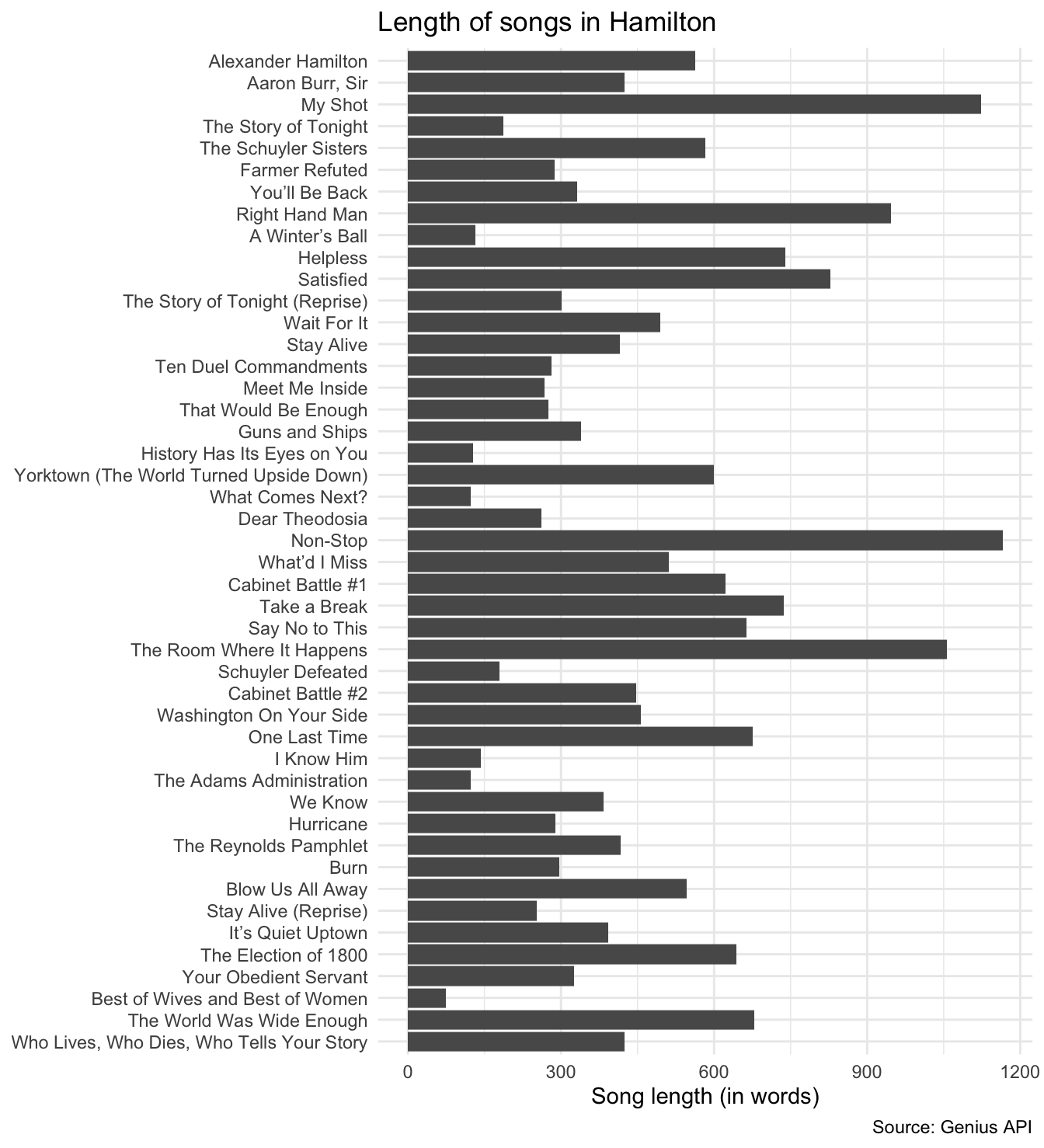
As a function of number of words, Non-Stop is the longest song in the musical.
Stop words
Of course not all words are equally important. Consider the 10 most frequent words in the lyrics:
hamilton_tidy %>%
  count(word) %>%
  arrange(desc(n))
## # A tibble: 2,929 × 2
##    word      n
##    <chr> <int>
##  1 the     848
##  2 i       639
##  3 you     578
##  4 to      544
##  5 a       471
##  6 and     383
##  7 in      317
##  8 it      294
##  9 of      274
## 10 my      259
## # … with 2,919 more rows
## # ℹ Use `print(n = ...)` to see more rows
Not particularly informative. We can identify a list of stopwords using get_stopwords() then remove them via anti_join().3
# remove stop words
hamilton_tidy <- hamilton_tidy %>%
  anti_join(get_stopwords(source = "smart"))
## Joining, by = "word"
hamilton_tidy %>%
  count(word) %>%
  slice_max(n = 20, order_by = n) %>%
  ggplot(aes(fct_reorder(word, n), n)) +
  geom_col() +
  coord_flip() +
  theme_minimal() +
  labs(
    title = "Frequency of Hamilton lyrics",
    x = NULL,
    y = NULL
  )
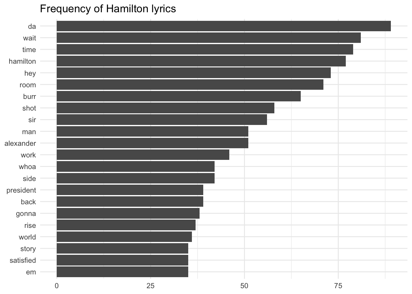
Now the words seem more relevant to the specific story being told in the musical.
Words used most by each cast member
Since we know which singer performs each line, we can examine the relative significance of different words to different characters. Term frequency-inverse document frequency (tf-idf) is a simple metric for measuring the importance of specific words to a corpus. Here let’s calculate the top ten words for each member of the principal cast.
# principal cast via Wikipedia
principal_cast <- c(
  "Hamilton", "Eliza", "Burr", "Angelica", "Washington",
  "Lafayette", "Jefferson", "Mulligan", "Madison",
  "Laurens", "Philip", "Peggy", "Maria", "King George"
)

# calculate tf-idf scores for words sung by the principal cast
hamilton_tf_idf <- hamilton_tidy %>%
  filter(speaker %in% principal_cast) %>%
  mutate(speaker = parse_factor(x = speaker, levels = principal_cast)) %>%
  count(speaker, word) %>%
  bind_tf_idf(term = word, document = speaker, n = n)

# visualize the top N terms per character by tf-idf score
hamilton_tf_idf %>%
  arrange(desc(tf_idf)) %>%
  mutate(word = factor(word, levels = rev(unique(word)))) %>%
  group_by(speaker) %>%
  slice_max(n = 10, order_by = tf_idf, with_ties = FALSE) %>%
  # resolve ambiguities when same word appears for different characters
  ungroup() %>%
  mutate(word = reorder_within(x = word, by = tf_idf, within = speaker)) %>%
  ggplot(mapping = aes(x = word, y = tf_idf)) +
  geom_col(show.legend = FALSE) +
  scale_x_reordered() +
  labs(
    title = "Most important words in *Hamilton*",
    subtitle = "Principal cast only",
    x = NULL,
    y = "tf-idf",
    caption = "Source: Genius API"
  ) +
  facet_wrap(facets = vars(speaker), scales = "free") +
  coord_flip() +
  theme(plot.title = element_markdown())
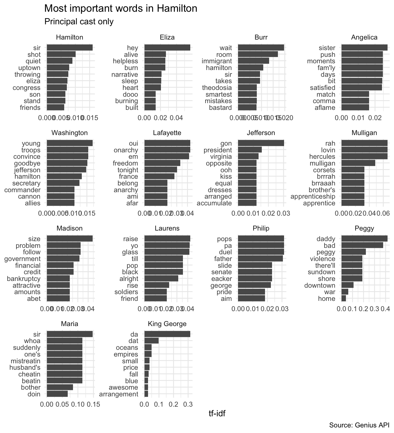
Again, some expected results stick out. Hamilton is always singing about not throwing away his shot, Eliza is helplessly in love with Alexander, while Burr regrets not being “in the room where it happens”. And don’t forget King George’s love songs to his wayward children.

Sentiment analysis
Sentiment analysis utilizes the text of the lyrics to classify content as positive or negative. Dictionary-based methods use pre-generated lexicons of words independently coded as positive/negative. We can combine one of these dictionaries with the Hamilton tidy-text data frame using inner_join() to identify words with sentimental affect, and further analyze trends.
Here we use the afinn dictionary which classifies 2,477 words on a scale of $[-5, +5]$.
# afinn dictionary
get_sentiments(lexicon = "afinn")
## # A tibble: 2,477 × 2
##    word       value
##    <chr>      <dbl>
##  1 abandon       -2
##  2 abandoned     -2
##  3 abandons      -2
##  4 abducted      -2
##  5 abduction     -2
##  6 abductions    -2
##  7 abhor         -3
##  8 abhorred      -3
##  9 abhorrent     -3
## 10 abhors        -3
## # … with 2,467 more rows
## # ℹ Use `print(n = ...)` to see more rows
hamilton_afinn <- hamilton_tidy %>%
  # join with sentiment dictionary
  inner_join(get_sentiments(lexicon = "afinn")) %>%
  # create row id and cumulative sentiment over the entire corpus
  mutate(
    cum_sent = cumsum(value),
    id = row_number()
  )
## Joining, by = "word"
hamilton_afinn
## # A tibble: 1,159 × 8
## song_number song_name line_num speaker word value cum_s…¹ id
## <dbl> <fct> <dbl> <chr> <chr> <dbl> <dbl> <int>
## 1 1 Alexander Hamilton 1 Aaron Burr bast… -5 -5 1
## 2 1 Alexander Hamilton 1 Aaron Burr whore -4 -9 2
## 3 1 Alexander Hamilton 2 Aaron Burr forg… -1 -10 3
## 4 1 Alexander Hamilton 4 Aaron Burr hero 2 -8 4
## 5 1 Alexander Hamilton 7 John Laure… smar… 2 -6 5
## 6 1 Alexander Hamilton 11 Thomas Jef… stru… -2 -8 6
## 7 1 Alexander Hamilton 12 Thomas Jef… long… -1 -9 7
## 8 1 Alexander Hamilton 13 Thomas Jef… steal -2 -11 8
## 9 1 Alexander Hamilton 17 James Madi… pain -2 -13 9
## 10 1 Alexander Hamilton 18 Burr insa… -2 -15 10
## # … with 1,149 more rows, and abbreviated variable name ¹cum_sent
## # ℹ Use `print(n = ...)` to see more rows
First, we can examine the sentiment of each song individually by calculating the average sentiment of each word in the song.
# sentiment by song
hamilton_afinn %>%
  group_by(song_name) %>%
  summarize(sent = mean(value)) %>%
  ggplot(mapping = aes(x = fct_rev(song_name), y = sent, fill = sent)) +
  geom_col() +
  scale_fill_viridis_c() +
  coord_flip() +
  labs(
    title = "Positive/negative sentiment in *Hamilton*",
    subtitle = "By song",
    x = NULL,
    y = "Average sentiment",
    fill = "Average\nsentiment",
    caption = "Source: Genius API"
  ) +
  theme(
    plot.title = element_markdown(),
    legend.position = "none"
  )
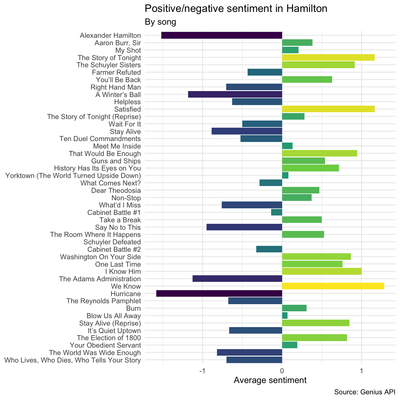
Again, the general themes of the songs come across in this analysis. “Alexander Hamilton” introduces Hamilton’s tragic backstory and difficult circumstances before emigrating to New York. “Dear Theodosia” is a love letter from Burr and Hamilton, promising to make the world a better place for their respective children.
However, this also illustrates some problems with dictionary-based sentiment analysis. Consider the back-to-back songs “Helpless” and “Satisfied”. “Helpless” depicts Eliza and Alexander falling in love with one another and getting married, while “Satisfied” recounts these same events from the perspective of Eliza’s sister Angelica who suppresses her own feelings for Hamilton out of a sense of duty to her sister. From the perspective of the listener, “Helpless” is the far more positive song of the pair. Why are they reversed based on the textual analysis?
get_sentiments(lexicon = "afinn") %>%
  filter(word %in% c("helpless", "satisfied"))
## # A tibble: 2 × 2
##   word      value
##   <chr>     <dbl>
## 1 helpless     -2
## 2 satisfied     2
Herein lies the problem with dictionary-based methods. The AFINN lexicon codes “helpless” as a negative term and “satisfied” as a positive term. On their own this makes sense, but in the context of the music clearly Eliza is “helplessly” in love while Angelica will in fact never be “satisfied” because she cannot be with Alexander. A dictionary-based sentiment classification will always miss these nuances in language.
We could also examine the general disposition of each speaker based on the sentiment of their lyrics. Consider the principal cast below:
hamilton_afinn %>%
  filter(speaker %in% principal_cast) %>%
  # calculate average sentiment by character with standard error
  group_by(speaker) %>%
  summarize(
    sent = mean(value),
    se = sd(value) / n()
  ) %>%
  # generate plot sorted from positive to negative
  ggplot(mapping = aes(x = fct_reorder(speaker, sent), y = sent, fill = sent)) +
  geom_pointrange(mapping = aes(
    ymin = sent - 2 * se,
    ymax = sent + 2 * se
  )) +
  coord_flip() +
  labs(
    title = "Positive/negative sentiment in *Hamilton*",
    subtitle = "By speaker",
    x = NULL,
    y = "Average sentiment",
    caption = "Source: Genius API"
  ) +
  theme(
    plot.title = element_markdown(),
    legend.position = "none"
  )
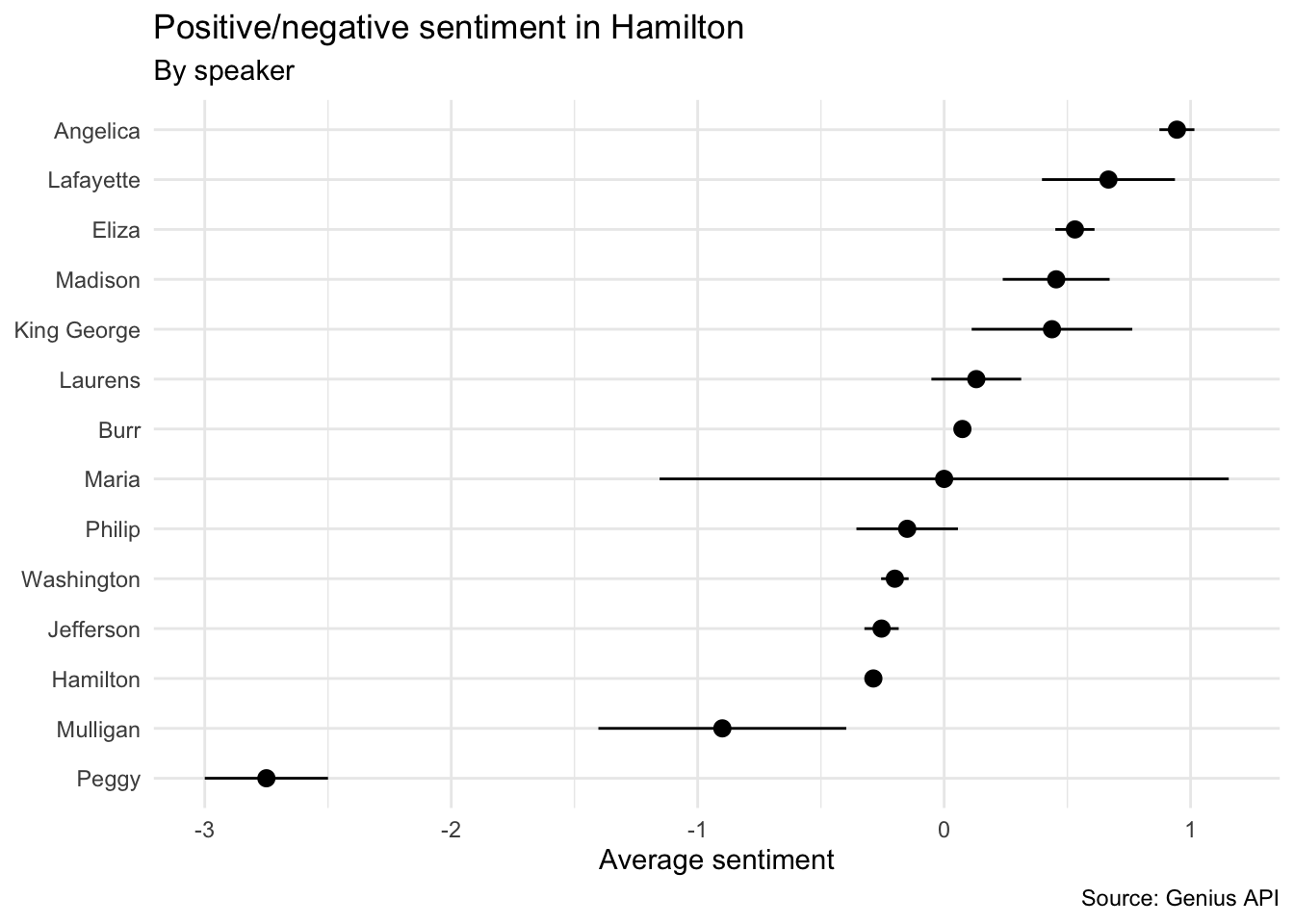
Given his generally neutral sentiment, Aaron Burr clearly follows his own guidance.
Also, can we please note Peggy’s general pessimism?
Tracking the cumulative sentiment across the entire musical, it’s easy to identify the high and low points.
ggplot(data = hamilton_afinn, mapping = aes(x = id, y = cum_sent)) +
  geom_line() +
  # label the start of each song
  scale_x_reverse(
    breaks = hamilton_afinn %>%
      group_by(song_number) %>%
      filter(id == min(id)) %>%
      pull(id),
    labels = hamilton_afinn %>%
      group_by(song_number) %>%
      filter(id == min(id)) %>%
      pull(song_name)
  ) +
  labs(
    title = "Positive/negative sentiment in *Hamilton*",
    x = NULL,
    y = "Cumulative sentiment",
    caption = "Source: Genius API"
  ) +
  # transpose to be able to fit song titles on the graph
  coord_flip() +
  theme(
    panel.grid.minor.y = element_blank(),
    plot.title = element_markdown()
  )
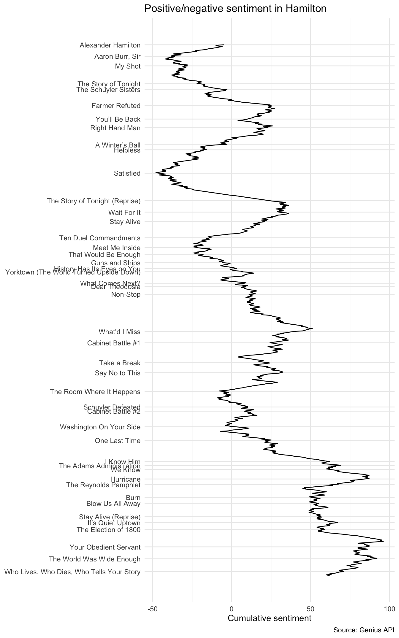
After the initial drop from “Alexander Hamilton”, the next peaks in the graph show several positive events in Hamilton’s life: meeting his friends, becoming Washington’s secretary, and meeting and marrying Eliza. The musical experiences a drop in tone during the rough years of the revolution and Hamilton’s dismissal back to New York, then rebounds as the revolutionaries close in on victory at Yorktown. Hamilton’s challenges as a member of Washington’s cabinet and rivalry with Jefferson are captured in the up-and-down swings in the graph, rises up with “One Last Time” and Hamilton writing Washington’s Farewell Address, dropping once again with “Hurricane” and the revelation of Hamilton’s affair, rising as Alexander and Eliza reconcile before finally descending once more upon Hamilton’s death in his duel with Burr.
Pairs of words
library(widyr)
library(ggraph)

# calculate all pairs of words in the musical
hamilton_pair <- hamilton %>%
  unnest_tokens(output = word, input = line, token = "ngrams", n = 2) %>%
  separate(col = word, into = c("word1", "word2"), sep = " ") %>%
  filter(
    !word1 %in% get_stopwords(source = "smart")$word,
    !word2 %in% get_stopwords(source = "smart")$word
  ) %>%
  drop_na(word1, word2) %>%
  count(word1, word2, sort = TRUE)

# filter for only relatively common combinations
bigram_graph <- hamilton_pair %>%
  filter(n > 3) %>%
  igraph::graph_from_data_frame()

# draw a network graph
set.seed(1776) # New York City
ggraph(bigram_graph, layout = "fr") +
  geom_edge_link(aes(edge_alpha = n, edge_width = n), show.legend = FALSE, alpha = .5) +
  geom_node_point(color = "#0052A5", size = 3, alpha = .5) +
  geom_node_text(aes(label = name), vjust = 1.5) +
  ggtitle("Word Network in Lin-Manuel Miranda's *Hamilton*") +
  theme_void() +
  theme(plot.title = element_markdown())
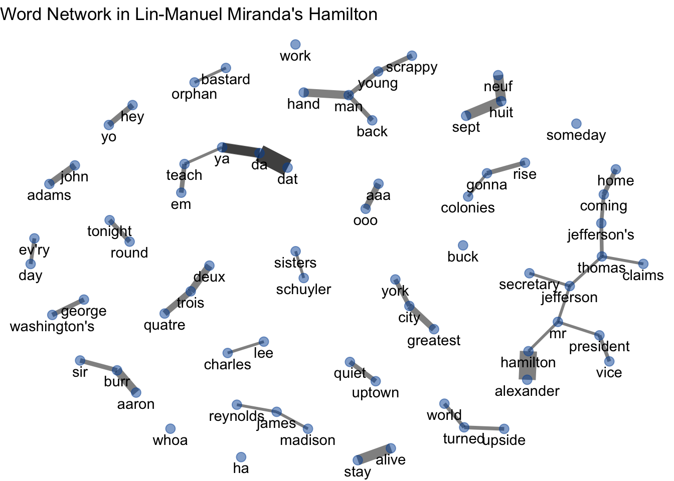
Finally we can examine the colocation of pairs of words to look for common usage. It’s apparent there are several major themes detected through this approach, including the Hamilton/Jefferson relationship, “Aaron Burr, sir”, Philip’s song with his mother (un, deux, trois, quatre, …), the rising up of the colonies, and those young, scrappy, and hungry men.
Acknowledgments
- This page is derived in part from A Sentiment Analysis of Hamilton: The broom Where it Happens / When are these #rcatladies gonna rise up? and licensed under a Creative Commons Attribution 4.0 International (CC BY 4.0) License.
- This page is derived in part from Alexander Hamilton: The Breakdown.
- This page is derived in part from Tidytext Analysis and licensed under a Creative Commons Attribution 4.0 International (CC BY 4.0) License.
Session Info
sessioninfo::session_info()
## ─ Session info ───────────────────────────────────────────────────────────────
##  setting  value
##  version  R version 4.2.1 (2022-06-23)
##  os       macOS Monterey 12.3
##  system   aarch64, darwin20
##  ui       X11
##  language (EN)
##  collate  en_US.UTF-8
##  ctype    en_US.UTF-8
##  tz       America/New_York
##  date     2022-08-22
##  pandoc   2.18 @ /Applications/RStudio.app/Contents/MacOS/quarto/bin/tools/ (via rmarkdown)
##
## ─ Packages ───────────────────────────────────────────────────────────────────
##  package       * version    date (UTC) lib source
##  assertthat      0.2.1      2019-03-21 [2] CRAN (R 4.2.0)
##  backports       1.4.1      2021-12-13 [2] CRAN (R 4.2.0)
##  blogdown        1.10       2022-05-10 [2] CRAN (R 4.2.0)
##  bookdown        0.27       2022-06-14 [2] CRAN (R 4.2.0)
##  broom           1.0.0      2022-07-01 [2] CRAN (R 4.2.0)
##  bslib           0.4.0      2022-07-16 [2] CRAN (R 4.2.0)
##  cachem          1.0.6      2021-08-19 [2] CRAN (R 4.2.0)
##  cellranger      1.1.0      2016-07-27 [2] CRAN (R 4.2.0)
##  cli             3.3.0      2022-04-25 [2] CRAN (R 4.2.0)
##  colorspace      2.0-3      2022-02-21 [2] CRAN (R 4.2.0)
##  crayon          1.5.1      2022-03-26 [2] CRAN (R 4.2.0)
##  curl            4.3.2      2021-06-23 [2] CRAN (R 4.2.0)
##  DBI             1.1.3      2022-06-18 [2] CRAN (R 4.2.0)
##  dbplyr          2.2.1      2022-06-27 [2] CRAN (R 4.2.0)
##  digest          0.6.29     2021-12-01 [2] CRAN (R 4.2.0)
##  dplyr         * 1.0.9      2022-04-28 [2] CRAN (R 4.2.0)
##  ellipsis        0.3.2      2021-04-29 [2] CRAN (R 4.2.0)
##  evaluate        0.16       2022-08-09 [1] CRAN (R 4.2.1)
##  fansi           1.0.3      2022-03-24 [2] CRAN (R 4.2.0)
##  farver          2.1.1      2022-07-06 [2] CRAN (R 4.2.0)
##  fastmap         1.1.0      2021-01-25 [2] CRAN (R 4.2.0)
##  forcats       * 0.5.1      2021-01-27 [2] CRAN (R 4.2.0)
##  fs              1.5.2      2021-12-08 [2] CRAN (R 4.2.0)
##  gargle          1.2.0      2021-07-02 [2] CRAN (R 4.2.0)
##  generics        0.1.3      2022-07-05 [2] CRAN (R 4.2.0)
##  geniusr       * 1.2.0      2020-04-13 [2] CRAN (R 4.2.0)
##  ggforce         0.3.3      2021-03-05 [2] CRAN (R 4.2.0)
##  ggplot2       * 3.3.6      2022-05-03 [2] CRAN (R 4.2.0)
##  ggraph        * 2.0.5      2021-02-23 [2] CRAN (R 4.2.0)
##  ggrepel         0.9.1      2021-01-15 [2] CRAN (R 4.2.0)
##  ggtext        * 0.1.1      2020-12-17 [2] CRAN (R 4.2.0)
##  glue            1.6.2      2022-02-24 [2] CRAN (R 4.2.0)
##  googledrive     2.0.0      2021-07-08 [2] CRAN (R 4.2.0)
##  googlesheets4   1.0.0      2021-07-21 [2] CRAN (R 4.2.0)
##  graphlayouts    0.8.0      2022-01-03 [2] CRAN (R 4.2.0)
##  gridExtra       2.3        2017-09-09 [2] CRAN (R 4.2.0)
##  gridtext        0.1.4      2020-12-10 [2] CRAN (R 4.2.0)
##  gtable          0.3.0      2019-03-25 [2] CRAN (R 4.2.0)
##  haven           2.5.0      2022-04-15 [2] CRAN (R 4.2.0)
##  here          * 1.0.1      2020-12-13 [2] CRAN (R 4.2.0)
##  hms             1.1.1      2021-09-26 [2] CRAN (R 4.2.0)
##  htmltools       0.5.3      2022-07-18 [2] CRAN (R 4.2.0)
##  httr            1.4.3      2022-05-04 [2] CRAN (R 4.2.0)
##  igraph          1.3.4      2022-07-19 [2] CRAN (R 4.2.0)
##  janeaustenr     0.1.5      2017-06-10 [2] CRAN (R 4.2.0)
##  jquerylib       0.1.4      2021-04-26 [2] CRAN (R 4.2.0)
##  jsonlite        1.8.0      2022-02-22 [2] CRAN (R 4.2.0)
##  knitr           1.39       2022-04-26 [2] CRAN (R 4.2.0)
##  lattice         0.20-45    2021-09-22 [2] CRAN (R 4.2.1)
##  lifecycle       1.0.1      2021-09-24 [2] CRAN (R 4.2.0)
##  lubridate       1.8.0      2021-10-07 [2] CRAN (R 4.2.0)
##  magrittr        2.0.3      2022-03-30 [2] CRAN (R 4.2.0)
##  MASS            7.3-58.1   2022-08-03 [2] CRAN (R 4.2.0)
##  Matrix          1.4-1      2022-03-23 [2] CRAN (R 4.2.1)
##  modelr          0.1.8      2020-05-19 [2] CRAN (R 4.2.0)
##  munsell         0.5.0      2018-06-12 [2] CRAN (R 4.2.0)
##  pillar          1.8.0      2022-07-18 [2] CRAN (R 4.2.0)
##  pkgconfig       2.0.3      2019-09-22 [2] CRAN (R 4.2.0)
##  polyclip        1.10-0     2019-03-14 [2] CRAN (R 4.2.0)
##  purrr         * 0.3.4      2020-04-17 [2] CRAN (R 4.2.0)
##  R6              2.5.1      2021-08-19 [2] CRAN (R 4.2.0)
##  rappdirs        0.3.3      2021-01-31 [2] CRAN (R 4.2.0)
##  Rcpp            1.0.9      2022-07-08 [2] CRAN (R 4.2.0)
##  readr         * 2.1.2      2022-01-30 [2] CRAN (R 4.2.0)
##  readxl          1.4.0      2022-03-28 [2] CRAN (R 4.2.0)
##  reprex          2.0.1.9000 2022-08-10 [1] Github (tidyverse/reprex@6d3ad07)
##  rlang           1.0.4      2022-07-12 [2] CRAN (R 4.2.0)
##  rmarkdown       2.14       2022-04-25 [2] CRAN (R 4.2.0)
##  rprojroot       2.0.3      2022-04-02 [2] CRAN (R 4.2.0)
##  rstudioapi      0.13       2020-11-12 [2] CRAN (R 4.2.0)
##  rvest           1.0.2      2021-10-16 [2] CRAN (R 4.2.0)
##  sass            0.4.2      2022-07-16 [2] CRAN (R 4.2.0)
##  scales          1.2.0      2022-04-13 [2] CRAN (R 4.2.0)
##  sessioninfo     1.2.2      2021-12-06 [2] CRAN (R 4.2.0)
##  SnowballC       0.7.0      2020-04-01 [2] CRAN (R 4.2.0)
##  stringi         1.7.8      2022-07-11 [2] CRAN (R 4.2.0)
##  stringr       * 1.4.0      2019-02-10 [2] CRAN (R 4.2.0)
##  textdata        0.4.2      2022-05-02 [2] CRAN (R 4.2.0)
##  tibble        * 3.1.8      2022-07-22 [2] CRAN (R 4.2.0)
##  tidygraph       1.2.1      2022-04-05 [2] CRAN (R 4.2.0)
##  tidyr         * 1.2.0      2022-02-01 [2] CRAN (R 4.2.0)
##  tidyselect      1.1.2      2022-02-21 [2] CRAN (R 4.2.0)
##  tidytext      * 0.3.3      2022-05-09 [2] CRAN (R 4.2.0)
##  tidyverse     * 1.3.2      2022-07-18 [2] CRAN (R 4.2.0)
##  tokenizers      0.2.1      2018-03-29 [2] CRAN (R 4.2.0)
##  tweenr          1.0.2      2021-03-23 [2] CRAN (R 4.2.0)
##  tzdb            0.3.0      2022-03-28 [2] CRAN (R 4.2.0)
##  utf8            1.2.2      2021-07-24 [2] CRAN (R 4.2.0)
##  vctrs           0.4.1      2022-04-13 [2] CRAN (R 4.2.0)
##  viridis         0.6.2      2021-10-13 [2] CRAN (R 4.2.0)
##  viridisLite     0.4.0      2021-04-13 [2] CRAN (R 4.2.0)
##  widyr         * 0.1.4      2021-08-12 [2] CRAN (R 4.2.0)
##  withr           2.5.0      2022-03-03 [2] CRAN (R 4.2.0)
##  xfun            0.31       2022-05-10 [1] CRAN (R 4.2.0)
##  xml2            1.3.3      2021-11-30 [2] CRAN (R 4.2.0)
##  yaml            2.3.5      2022-02-21 [2] CRAN (R 4.2.0)
##
##  [1] /Users/soltoffbc/Library/R/arm64/4.2/library
##  [2] /Library/Frameworks/R.framework/Versions/4.2-arm64/Resources/library
##
## ──────────────────────────────────────────────────────────────────────────────
There are a number of ways to obtain the lyrics for the entire soundtrack. One approach is to use
rvestand web scraping to extract the lyrics from sources online. However here I used the Genius API andgeniusrto systematically collect the lyrics from an authoritative (and legal) source. The code below was used to obtain the lyrics for all the songs. Note that you need to authenticate using an API token in order to use this code.↩︎library(geniusr) # Genius album ID number hamilton_id <- 131575 # retrieve track list hamilton_tracks <- get_album_tracklist_id(album_id = hamilton_id) # retrieve song lyrics hamilton_lyrics <- hamilton_tracks %>% mutate(lyrics = map(.x = song_lyrics_url, get_lyrics_url)) # unnest and clean-up hamilton <- hamilton_lyrics %>% unnest(cols = lyrics, names_repair = "universal") %>% select(song_number, line, section_name, song_name) %>% group_by(song_number) %>% # add line number mutate(line_num = row_number()) %>% # reorder columns and convert speaker to title case select(song_number, song_name, line_num, line, speaker = section_name) %>% mutate( speaker = str_to_title(speaker), line = str_replace_all(line, "’", "'") ) %>% # write to disk write_csv(path = here("static", "data", "hamilton.csv")) glimpse(hamilton)Though lyrics’ length is not always a good measure of a musical’s pacing. ↩︎
I told you filtering joins would be useful one day, but you didn’t believe me! ↩︎