Building Shiny applications
library(tidyverse)
library(shiny)
Shiny is a package from RStudio that can be used to build interactive web pages with R. While that may sound scary because of the words “web pages”, it’s geared to R users who have no experience with web development, and you do not need to know any HTML/CSS/JavaScript.
You can do quite a lot with Shiny: think of it as an easy way to make an interactive web page, and that web page can seamlessly interact with R and display R objects (plots, tables, of anything else you do in R). To get a sense of the wide range of things you can do with Shiny, you can visit the Shiny gallery, which hosts examples of basic (and complex) Shiny apps.
In this lesson, we’ll walk through all the steps of building a Shiny app using a subset of the city of Chicago’s current employee data set. The city annually releases an updated file of all employees of the city government, including information on department, job title, and salary/wage. We will build an app to report information specifically for wage employees. The final version of the app can be seen here. Any activity deemed as an exercise throughout this tutorial is not mandatory for building our app, but they are good for getting more practice with Shiny.
If you want even more practice, another great tutorial is the official Shiny tutorial. RStudio also provides a handy cheatsheet to remember all the little details after you already learned the basics.
Before we begin
You’ll need to have the shiny package, so install it.
install.packages("shiny")
To ensure you successfully installed Shiny, try running one of the demo apps.
library(shiny)
runExample("01_hello")
If the example app is running, press Escape to close the app, and you are ready to build your first Shiny app!
To follow along with this lesson, fork and clone the shiny-demo Git repository which contains the data files for city employees.
Shiny app basics
Every Shiny app is composed of a two parts: a web page that shows the app to the user, and a computer that powers the app. The computer that runs the app can either be your own laptop (such as when you’re running an app from RStudio) or a server somewhere else. You, as the Shiny app developer, need to write these two parts (you’re not going to write a computer, but rather the code that powers the app). In Shiny terminology, they are called UI (user interface) and server.
UI is just a web document that the user gets to see, it’s HTML that you write using Shiny’s functions. The UI is responsible for creating the layout of the app and telling Shiny exactly where things go. The server is responsible for the logic of the app; it’s the set of instructions that tell the web page what to show when the user interacts with the page.
If you look at the app we will be building, the page that you see is built with the UI code. You’ll notice there are some controls that you, as the user, can manipulate. If you adjust the price or choose a type of alcohol, you’ll notice that the plot and the table get updated. The UI is responsible for creating these controls and telling Shiny where to place the controls and where to place the plot and table, while the server is responsible for creating the actual plot or the data in the table.
Create an empty Shiny app
All Shiny apps follow the same template:
library(shiny)
ui <- fluidPage()
server <- function(input, output) {}
shinyApp(ui = ui, server = server)
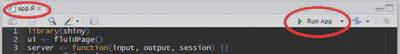
This template is by itself a working minimal Shiny app that doesn’t do much. It initializes an empty UI and an empty server, and runs an app using these empty parts. Copy this template into a new file named app.R in a new folder. It is very important that the name of the file is app.R, otherwise it would not be recognized as a Shiny app. It is also very important that you place this app in its own folder, and not in a folder that already has other R scripts or files, unless those other files are used by your app.
After saving the file, RStudio should recognize that this is a Shiny app, and you should see the usual Run button at the top change to Run App.
If you don’t see the Run App button, it means you either have a very old version of RStudio, don’t have Shiny installed, or didn’t follow the file naming conventions.
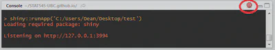
Click the Run App button, and now your app should run. You won’t see much because it’s an empty app, but you should see that the console has some text printed in the form of Listening on http://127.0.0.1:5274 and that a little stop sign appeared at the top of the console. You’ll also notice that you can’t run any commands in the console. This is because R is busy–your R session is currently powering a Shiny app and listening for user interaction (which won’t happen because the app has nothing in it yet).
Click the stop button to stop the app, or press the Escape key.
You may have noticed that when you click the Run App button, all it’s doing is just running the function shiny::runApp() in the console. You can run that command instead of clicking the button if you prefer.
Exercise: Try running the empty app using the runApp() function instead of using the Run App button.
Alternate way to create a Shiny app: separate UI and server files
Another way to define a Shiny app is by separating the UI and server code into two files: ui.R and server.R. This is the preferable way to write Shiny apps when the app is complex and involves more code, but in this tutorial we’ll stick to the simple single file. If you want to break up your app into these two files, you simply put all code that is assigned to the ui variable in ui.R and all the code assigned to the server function in server.R. When RStudio sees these two files in the same folder, it will know you’re writing a Shiny app.
Exercise: Try making a new Shiny app by creating the two files ui.R and server.R. Remember that they have to be in the same folder. Also remember to put them in a new, isolated folder (not where your app.R already exists).
Let RStudio fill out a Shiny app template for you
You can also create a new Shiny app using RStudio’s menu by selecting File > New File > Shiny Web App…. If you do this, RStudio will let you choose if you want a single-file app (app.R) or a two-file app (ui.R+server.R). RStudio will initialize a simple functional Shiny app with some code in it. I personally don’t use this feature because I find it easier to simply type the few lines of a Shiny app and save the files.
Load the dataset
The raw dataset contains information about all employees of the city of Chicago (employees-all.csv). The processed dataset we’ll be using in this app is the subset of employees who are wage employees (paid hourly), as opposed to salaried employees. This subset is in the employees-wage.csv file.1
Add a line in your app to load the data into a variable called employ. It should look something like this (be sure to to add library(tidyverse) or library(readr) to the script so you can use the read_csv function):
employ <- read_csv("employees-wage.csv")
Place this line in your app as the third line, just after library(shiny) and library(tidyverse). Make sure the file path and file name are correct, otherwise your app won’t run. Try to run the app to make sure the file can be loaded without errors.
If you want to verify that the app can successfully read the data, you can add a print() statement after reading the data. This won’t make anything happen in your Shiny app, but you will see a summary of the dataset printed in the console, which should let you know that the dataset was indeed loaded correctly. You can place the following line after reading the data:
print(glimpse(employ))
Once you get confirmation that the data is properly loaded, you can remove that line.
Exercise: Load the data file into R and get a feel for what’s in it. How big is it, what variables are there, what are the normal wage ranges, etc.
Build the basic UI
Let’s start populating our app with some elements visually. This is usually the first thing you do when writing a Shiny app - add elements to the UI.
Add plain text to the UI
You can place R strings inside fluidPage() to render text.
fluidPage("City of Chicago Wage Employees", "hourly wage")
Replace the line in your app that assigns an empty fluidPage() into ui with the one above, and run the app.
The entire UI will be built by passing comma-separated arguments into the fluidPage() function. By passing regular text, the web page will just render boring unformatted text.
Exercise: Add several more strings to fluidPage() and run the app. Nothing too exciting is happening yet, but you should just see all the text appear in one contiguous block.
Add formatted text and other HTML elements
If we want our text to be formatted nicer, Shiny has many functions that are wrappers around HTML tags that format text. We can use the h1() function for a top-level header (<h1> in HTML), h2() for a secondary header (<h2> in HTML), strong() to make text bold (<strong> in HTML), em() to make text italicized (<em> in HTML), and many more.
There are also functions that are wrappers to other HTML tags, such as br() for a line break, img() for an image, a() for a hyperlink, and others.
All of these functions are actually just wrappers to HTML tags with the equivalent name. You can add any arbitrary HTML tag using the tags object, which you can learn more about by reading the help file on tags.
Just as a demonstration, try replacing the fluidPage() function in your UI with
ui <- fluidPage(
  h1("My app"),
  "Chicago",
  "Wage Employees",
  br(),
  "Hourly",
  strong("wage")
)
Run the app with this code as the UI. Notice the formatting of the text and understand why it is rendered that way.
div("this is blue", style = "color: blue;").Exercise: Experiment with different HTML-wrapper functions inside fluidPage(). Run the fluidPage(...) function in the console and see the HTML that it creates.
Add a title
We could add a title to the app with h1(), but Shiny also has a special function titlePanel(). Using titlePanel() not only adds a visible big title-like text to the top of the page, but it also sets the “official” title of the web page. This means that when you look at the name of the tab in the browser, you’ll see this title.
Overwrite the fluidPage() that you experimented with so far, and replace it with the simple one below, that simply has a title and nothing else.
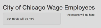
fluidPage(
  titlePanel("City of Chicago Wage Employees")
)
Exercise: Look at the documentation for the titlePanel() function and notice it has another argument. Use that argument and see if you can see what it does.
Add a layout
You may have noticed that so far, by just adding text and HTML tags, everything is unstructured and the elements simply stack up one below the other in one column. We’ll use sidebarLayout() to add a simple structure. It provides a simple two-column layout with a smaller sidebar and a larger main panel. We’ll build our app such that all the inputs that the user can manipulate will be in the sidebar, and the results will be shown in the main panel on the right.
Add the following code after the titlePanel()
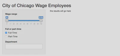
sidebarLayout(
  sidebarPanel("our inputs will go here"),
  mainPanel("the results will go here")
)
Remember that all the arguments inside fluidPage() need to be separated by commas.
So far our complete app looks like this (hopefully this isn’t a surprise to you)
library(shiny)
library(tidyverse)

employ <- read_csv("employees-wage.csv")

ui <- fluidPage(
  titlePanel("City of Chicago Wage Employees"),
  sidebarLayout(
    sidebarPanel("our inputs will go here"),
    mainPanel("the results will go here")
  )
)

server <- function(input, output) {}

shinyApp(ui = ui, server = server)
?column and ?fluidRow.Exercise: Add some UI into each of the two panels (sidebar panel and main panel) and see how your app now has two columns.
All UI functions are simply HTML wrappers
This was already mentioned, but it’s important to remember: the entire UI is just HTML, and Shiny simply gives you easy tools to write it without having to know HTML. To convince yourself of this, look at the output when printing the contents of the ui variable.
print(ui)
<div class="container-fluid">
  <h2>City of Chicago Wage Employees</h2>
  <div class="row">
    <div class="col-sm-4">
      <form class="well">our inputs will go here</form>
    </div>
    <div class="col-sm-8">the results will go here</div>
  </div>
</div>
This should make you appreciate Shiny for not making you write horrendous HTML by hand.
Add inputs to the UI
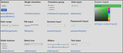
Inputs are what gives users a way to interact with a Shiny app. Shiny provides many input functions to support many kinds of interactions that the user could have with an app. For example, textInput() is used to let the user enter text, numericInput() lets the user select a number, dateInput() is for selecting a date, selectInput() is for creating a select box (aka a dropdown menu).
All input functions have the same first two arguments: inputId and label. The inputId will be the name that Shiny will use to refer to this input when you want to retrieve its current value. It is important to note that every input must have a unique inputId. If you give more than one input the same id, Shiny will unfortunately not give you an explicit error, but your app won’t work correctly. The label argument specifies the text in the display label that goes along with the input widget. Every input can also have multiple other arguments specific to that input type. The only way to find out what arguments you can use with a specific input function is to look at its help file.
Exercise: Read the documentation of ?numericInput and try adding a numeric input to the UI. Experiment with the different arguments. Run the app and see how you can interact with this input. Then try different inputs types.
Input for hourly wage
The first input we want to have is for specifying a wage range (minimum and maximum hourly wage). The most sensible types of input for this are either numericInput() or sliderInput() since they are both used for selecting numbers. If we use numericInput(), we’d have to use two inputs, one for the minimum value and one for the maximum. Looking at the documentation for sliderInput(), you’ll see that by supplying a vector of length two as the value argument, it can be used to specify a range rather than a single number. This sounds like what we want in this case, so we’ll use sliderInput().
To create a slider input, a maximum value needs to be provided. We could manually determine the highest hourly wage rate in the dataset and hardcode this into the app. But we’re already using R, so let’s calculate it dynamically. That is, write a short piece of R code to determine the largest value in the wage column. max() does exactly that.
max(employ$wage, na.rm = TRUE)
## [1] 109
By looking at the documentation for the slider input function, the following piece of code can be constructed.
sliderInput(inputId = "wage",
            label = "Wage range",
            min = 0,
            max = max(employ$wage, na.rm = TRUE),
            value = c(0, max(employ$wage, na.rm = TRUE)),
            pre = "$")
Place the code for the slider input inside sidebarPanel() (replace the text we wrote earlier with this input).
Exercise: Run the code of the sliderInput() in the R console and see what it returns. Change some of the parameters of sliderInput(), and see how that changes the result. It’s important to truly understand that all these functions in the UI are simply a convenient way to write HTML, as is apparent whenever you run these functions on their own.
Input for full/part-time
While many employees of the city are full-time workers, a large portion only work for the city part-time. Part-time workers are more likely to be seasonal employees, and as such their hourly wages may systematically differ from full-time employees. It will be helpful to include an option to filter the datset between these two types of employees.
For this we want some kind of a text input. But allowing the user to enter text freely isn’t the right solution because we want to restrict the user to only two choices. We could either use radio buttons or a select box for our purpose. Let’s use radio buttons for now since there are only two options, so take a look at the documentation for radioButtons() and come up with a reasonable input function code. It should look like this:
radioButtons(inputId = "full_time",
             label = "Full or part-time",
             choices = c("Full-Time", "Part-Time"))
Add this input code inside sidebarPanel(), after the previous input (separate them with a comma).
Input for department
Different departments will offer different wage structures depending on the value of the skills in demand. The city classifies wage employees into 22 distinct departments:
| Department | Number of Employees |
|---|---|
| Animal Care and Control | 19 |
| Aviation | 1082 |
| Budget & Management | 2 |
| Business Affairs and Consumer Protection | 7 |
| City Council | 64 |
| Community Development | 4 |
| Cultural Affairs and Special Events | 7 |
| Emergency Management & Communications | 1273 |
| Family & Support | 287 |
| Finance | 44 |
| Fire | 2 |
| General Services | 765 |
| Human Resources | 4 |
| Law | 40 |
| Mayor’s Office | 8 |
| Police | 10 |
| Procurement Services | 2 |
| Public Health | 3 |
| Public Library | 299 |
| Streets & Sanitation | 1862 |
| Transportation | 725 |
| Water Management | 1513 |
The most appropriate input type in this case is probably the select box selectInput(). However we don’t want to write out the entire vector by hand:
## c("Animal Care and Control", "Aviation", "Budget & Management", "Business Affairs and Consumer Protection", "City Council", "Community Development", "Cultural Affairs and Special Events", "Emergency Management & Communications", "Family & Support", "Finance", "Fire", "General Services", "Human Resources", "Law", "Mayor's Office", "Police", "Procurement Services", "Public Health", "Public Library", "Streets & Sanitation", "Transportation", "Water Management")
Instead, like before we’ll extract these values directly from the data frame:
selectInput(inputId = "department",
            label = "Department",
            choices = sort(unique(employ$department)),
            multiple = TRUE)
multiple = TRUE so the user can select more than one department at a time.Add this function as well to your app. If you followed along, your entire app should have this code:
library(shiny)
library(tidyverse)

employ <- read_csv("employees-wage.csv")

ui <- fluidPage(
  titlePanel("City of Chicago Wage Employees"),
  sidebarLayout(
    sidebarPanel(
      sliderInput(inputId = "wage",
                  label = "Wage range",
                  min = 0,
                  max = max(employ$wage, na.rm = TRUE),
                  value = c(0, max(employ$wage, na.rm = TRUE)),
                  pre = "$"),
      radioButtons(inputId = "full_time",
                   label = "Full or part-time",
                   choices = c("Full-Time", "Part-Time")),
      selectInput(inputId = "department",
                  label = "Department",
                  choices = sort(unique(employ$department)),
                  multiple = TRUE)
    ),
    mainPanel("the results will go here")
  )
)

server <- function(input, output) {}

shinyApp(ui = ui, server = server)
Add placeholders for outputs
After creating all the inputs, we should add elements to the UI to display the outputs. Outputs can be any object that R creates and that we want to display in our app - such as a plot, a table, or text. We’re still only building the UI, so at this point we can only add placeholders for the outputs that will determine where an output will be and what its ID is, but it won’t actually show anything. Each output needs to be constructed in the server code later.
Shiny provides several output functions, one for each type of output. Similarly to the input functions, all the output functions have an outputId argument that is used to identify each output, and this argument must be unique for each output.
Output for a plot of the results
At the top of the main panel we’ll have a plot showing the distribution of hourly wages. Since we want a plot, the function we use is plotOutput().
Add the following code into the mainPanel() (replace the existing text):
plotOutput("hourlyPlot")
This will add a placeholder in the UI for a plot named hourlyPlot.
Exercise: To remind yourself that we are still merely constructing HTML and not creating actual plots yet, run the above plotOutput() function in the console to see that all it does is create some HTML.
Output for a table summary of the results
Below the plot, we will have a table that shows a summary of the number of employees per department currently included in the plot. To get a table, we use the tableOutput() function.
Here is a simple way to create a UI element that will hold a table output:
tableOutput("employTable")
Add this output to the mainPanel() as well. Maybe add a couple br() in between the two outputs, just as a space buffer so that they aren’t too close to each other.
Checkpoint: what our app looks like after implementing the UI
If you’ve followed along, your app should now have this code:
library(shiny)
library(tidyverse)

employ <- read_csv("employees-wage.csv")

ui <- fluidPage(
  titlePanel("City of Chicago Wage Employees"),
  sidebarLayout(
    sidebarPanel(
      sliderInput(inputId = "wage",
                  label = "Wage range",
                  min = 0,
                  max = max(employ$wage, na.rm = TRUE),
                  value = c(0, max(employ$wage, na.rm = TRUE)),
                  pre = "$"),
      radioButtons(inputId = "full_time",
                   label = "Full or part-time",
                   choices = c("Full-Time", "Part-Time")),
      selectInput(inputId = "department",
                  label = "Department",
                  choices = sort(unique(employ$department)),
                  multiple = TRUE)
    ),
    mainPanel(plotOutput("hourlyPlot"),
              tableOutput("employTable"))
  )
)

server <- function(input, output) {}

shinyApp(ui = ui, server = server)
Implement server logic to create outputs
So far we only wrote code inside that was assigned to the ui variable (or code that was written in ui.R). That’s usually the easier part of a Shiny app. Now we have to write the server function, which will be responsible for listening to changes to the inputs and creating outputs to show in the app.
If you look at the server function, you’ll notice that it is always defined with two arguments: input and output. You must define these two arguments! Both input and output are list-like objects. As the names suggest, input is a list you will read values from and output is a list you will write values to. input will contain the values of all the different inputs at any given time, and output is where you will save output objects (such as tables and plots) to display in your app.
Building an output
Recall that we created two output placeholders: hourlyPlot (a plot) and employTable (a table). We need to write code in R that will tell Shiny what kind of plot or table to display. There are three rules to build an output in Shiny.
- Save the output object into the
outputlist (remember the app template - every server function has anoutputargument) - Build the object with a
render*function, where*is the type of output - Access input values using the
inputlist (every server function has aninputargument)
The third rule is only required if you want your output to depend on some input, so let’s first see how to build a very basic output using only the first two rules. We’ll create a plot and send it to the hourlyPlot output.
output$hourlyPlot <- renderPlot({
  plot(rnorm(100))
})
This simple code shows the first two rules: we’re creating a plot inside the renderPlot() function, and assigning it to hourlyPlot in the output list. Remember that every output created in the UI must have a unique ID, now we see why. In order to attach an R object to an output with ID x, we assign the R object to output$x.
Since hourlyPlot was defined as a plotOutput, we must use the renderPlot function, and we must create a plot inside the renderPlot function.
If you add the code above inside the server function, you should see a plot with 100 random points in the app.
Exercise: The code inside renderPlot() doesn’t have to be only one line, it can be as long as you’d like as long as it returns a plot. Try making a more complex plot using ggplot2. The plot doesn’t have to use our dataset, it could be anything, just to make sure you can use renderPlot().
Making an output react to an input
Now we’ll take the plot one step further. Instead of always plotting the same plot (100 random numbers), let’s use the minimum wage selected as the number of points to show. It doesn’t make too much sense, but it’s just to learn how to make an output depend on an input.
output$hourlyPlot <- renderPlot({
  plot(rnorm(input$wage[1]))
})
Replace the previous code in your server function with this code, and run the app. Whenever you choose a new minimum price range, the plot will update with a new number of points. Notice that the only thing different in the code is that instead of using the number 100 we are using input$wage[1].
What does this mean? Just like the variable output contains a list of all the outputs (and we need to assign code into them), the variable input contains a list of all the inputs that are defined in the UI. input$wage return a vector of length 2 containing the minimum and maximum wage. Whenever the user manipulates the slider in the app, these values are updated, and whatever code relies on it gets re-evaluated. This is a concept known as reactivity, which we will get to in a few minutes.
Notice that these short 3 lines of code are using all the 3 rules for building outputs: we are saving to the output list (output$hourlyPlot <-), we are using a render* function to build the output (renderPlot({})), and we are accessing an input value (input$wage[1]).
Building the plot output
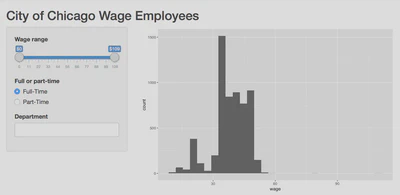
Now we have all the knowledge required to build a plot visualizing some aspect of the data. We’ll create a simple histogram of the hourly wage rate for employees by using the same 3 rules to create a plot output.
First we need to make sure ggplot2 is loaded, so add a library(ggplot2) at the top (or just continue to use library(tidyverse).
Next we’ll return a histogram of hourly wage wage from renderPlot(). Let’s start with just a histogram of the whole data, unfiltered.
output$hourlyPlot <- renderPlot({
  ggplot(employ, aes(wage)) +
    geom_histogram()
})
If you run the app with this code inside your server, you should see a histogram in the app. But if you change the input values, nothing happens yet, so the next step is to actually filter the dataset based on the inputs.
Recall that we have 3 inputs: wage, full_time, and department. We can filter the data based on the values of these three inputs. For now, only filter for wage and full_time – we’ll return to department in a little bit. We’ll use dplyr functions to filter the data, so be sure to include library(dplyr) at the top. Then we’ll plot the filtered data instead of the original data.
output$hourlyPlot <- renderPlot({
  employ %>%
    filter(full_time == input$full_time,
           wage >= input$wage[[1]],
           wage <= input$wage[[2]]) %>%
    ggplot(aes(wage)) +
    geom_histogram()
})
Place this code in your server function and run the app. If you change the hourly wage or full/part-time inputs, you should see the histogram update.
Read this code and understand it. You’ve successfully created an interactive app - the plot is changing according to the user’s selection.
To make sure we’re on the same page, here is what your code should look like at this point:
library(shiny)
library(tidyverse)

employ <- read_csv("employees-wage.csv")

ui <- fluidPage(
  titlePanel("City of Chicago Wage Employees"),
  sidebarLayout(
    sidebarPanel(
      sliderInput(inputId = "wage",
                  label = "Wage range",
                  min = 0,
                  max = max(employ$wage, na.rm = TRUE),
                  value = c(0, max(employ$wage, na.rm = TRUE)),
                  pre = "$"),
      radioButtons(inputId = "full_time",
                   label = "Full or part-time",
                   choices = c("Full-Time", "Part-Time")),
      selectInput(inputId = "department",
                  label = "Department",
                  choices = sort(unique(employ$department)),
                  multiple = TRUE)
    ),
    mainPanel(plotOutput("hourlyPlot"),
              tableOutput("employTable"))
  )
)

server <- function(input, output) {
  output$hourlyPlot <- renderPlot({
    employ %>%
      filter(full_time == input$full_time,
             wage >= input$wage[[1]],
             wage <= input$wage[[2]]) %>%
      ggplot(aes(wage)) +
      geom_histogram()
  })
}

shinyApp(ui = ui, server = server)
Exercise: The current plot doesn’t look very nice, you could enhance the plot and make it much more pleasant to look at.
Building the table output
Building the next output should be much easier now that we’ve done it once. The other output we have was called employTable (as defined in the UI) and should be a table summarizing the number of employees per department in the filtered data frame. Since it’s a table output, we should use the renderTable() function. We’ll do the exact same filtering on the data, and then simply return the summarized data as a data.frame. Shiny will know that it needs to display it as a table because it’s defined as a tableOutput.
The code for creating the table output should make sense to you without too much explanation:
output$employTable <- renderTable({
  employ %>%
    filter(full_time == input$full_time,
           wage >= input$wage[[1]],
           wage <= input$wage[[2]]) %>%
    count(department)
})
Add this code to your server. Don’t overwrite the previous definition of output$hourlyPlot, just add this code before or after that, but inside the server function. Run your app, and be amazed! You can now see a table showing the number of wage employees per department that match your criteria.
ui, we are using a predefined function called fluidPage() so all of our different elements for the UI are separated by commas. This is because each element for the page is an argument for the fluidPage() function. In building server, we are writing a new function. For this reason we don’t have to separate each element with a comma. We just write it like we would any other function!Exercise: Add a new output. Either a new plot, a new table, or some piece of text that changes based on the inputs. For example, you could add a text output (textOutput() in the UI, renderText() in the server) that says how many results were found. If you choose to do this, I recommend first adding the output to the UI, then building the output in the server with static text to make sure you have the syntax correct. Only once you can see the text output in your app you should make it reflect the inputs. Pro-tip: since textOutput() is written in the UI, you can wrap it in other UI functions. For example, h2(textOutput(...)) will result in larger text.
Reactivity 101
Shiny uses a concept called reactive programming. This is what enables your outputs to react to changes in inputs. Reactivity in Shiny is complex, but as an extreme oversimplification, it means that when the value of a variable x changes, then anything that relies on x gets re-evaluated. Notice how this is very different from what you are used to in R. Consider the following code:
x <- 5
y <- x + 1
x <- 10
What is the value of y? It’s 6. But in reactive programming, if x and y are reactive variables, then the value of y would be 11 because it would be updated whenever x is changed. This is a very powerful technique that is very useful for creating the responsiveness of Shiny apps, but it might be a bit weird at first because it’s a very different concept from what you’re used to.
Only reactive variables behave this way, and in Shiny all inputs are automatically reactive. That’s why you can always use input$x in render functions, and you can be sure that whatever output depends on x will use the updated value of x whenever x changes.
You might be wondering what it means to “depend” on a variable. This is not the official terminology, but it simply means that the variable is referenced in the code. So by merely accessing the value of a reactive variable, it causes the current code block to “depend” on that variable. Consider the following sample code to create a plot with a specific number of points in a specific color:
output$someoutput <- renderPlot({
  col <- input$mycolor
  num <- input$mynumber
  plot(rnorm(num), col = col)
})
The above render function accesses two different inputs: input$mycolor and input$mynumber. This means that this code block depends on both of these variables, so whenever either one of the two inputs is updated, the code gets re-executed with the new input values and output$someoutput is updated.
Creating and accessing reactive variables
One very important thing to remember about reactive variables (such as the input list) is that they can only be used inside reactive contexts. Any render* function is a reactive context, so you can always use input$x or any other reactive variable inside render functions. There are two other common reactive contexts that we’ll get to in a minute: reactive({}) and observe({}). To show you what this means, let’s try accessing the price input value in the server function, without explicitly being inside a reactive context. Simply add print(input$wage) inside the server function, and you will get an error when running the app:
Operation not allowed without an active reactive context. (You tried to do something that can only be done from inside a reactive expression or observer.)
Shiny is very clear about what the error is: we are trying to access a reactive variable outside of a reactive context. To fix this, we can use the observe({}) function to access the input variable. Inside the server, replace print(input$wage) with observe({ print(input$wage) }), and now the app should run fine. Note that this observe({}) statement depends on input$wage, so whenever you change the value of the price, the code inside this observe({}) will run again, and the new value will be printed. This is actually a very simple yet useful debugging technique in Shiny: often you want to know what value a reactive variable holds, so you need to remember to wrap the cat(input$x) or print(input$x) by an observe({}).
So far we only saw one reactive variable: the input list. You can also create your own reactive variables using the reactive({}) function. The reactive({}) function is similar to observe({}) in that it is also a reactive context, which means that it will get re-run whenever any of the reactive variables in it get updated. The difference between them is that reactive({}) returns a value. To see it in action, let’s create a variable called wageDiff that will be the difference between the maximum and minimum wage selected. If you try to naively define wageDiff <- diff(input$wage), you’ll see the same error as before about doing something outside a reactive context. This is because input$wage is a reactive variable, and we can’t use a reactive variable outside a reactive context. Since we want to assign a value, we use the reactive({}) function. Try adding the following line to your server:
wageDiff <- reactive({
  diff(input$wage)
})
Now your app will run. If you want to access a reactive variable defined with reactive({}), you must add parentheses after the variable name, as if it’s a function. To demonstrate this, add observe({ print(wageDiff()) }) to your server function. Notice that we use wageDiff() rather than wageDiff. It’s very important to remember this, because you can get confusing unclear errors if you simply try to access a custom reactive variable without the parentheses.
You can think of reactivity as causing a chain reaction: when one reactive value changes, anything that depends on it will get updated. If any of the updated values are themselves reactive variables, then any reactive contexts that depend on those variables will also get updated in turn. As a concrete example, let’s think about what happens when you change the value of the wage on the page. Since input$wage is a reactive variable, any expression that uses it will get updated. This means the two render functions from earlier will execute because they both depend on input$wage, as well as the wageDiff variable because it also depends on it. But since wageDiff is itself a reactive variable, Shiny will check if there is anything that depends on wageDiff, and indeed there is - the observe({}) function that prints the value of wageDiff. So once wageDiff gets updated, the observe({}) function will run, and the value will get printed.
Reactivity is usually the hardest part about Shiny to understand, so if you don’t quite get it, don’t feel bad. Try reading this section again, and I promise that with time and experience you will get more comfortable with reactivity. Once you do feel more confident with reactivity, it may be a good idea to read more advanced documentation describing reactivity, since this section greatly simplifies ideas to make them more understandable. A great resource is RStudio’s tutorial on reactivity.
Before continuing to the next section, you can remove all the observe({}) and reactive({}) functions we wrote in this section since they were all just for learning purposes.
Exercise: Read this section again and really understand what a reactive variable means, what the 3 main reactive contexts are, how you can define reactive variables, and how a reactivity chain of events works.
Using reactive variables to reduce code duplication
You may have noticed that we have the exact same code filtering the dataset in two places, once in each render function. We can solve that problem by defining a reactive variable that will hold the filtered dataset, and use that variable in the render functions.
The first step would be to create the reactive variable. The following code should be added to the server() function.
employ_filter <- reactive({
  employ %>%
    filter(
      # filter by full or part-time
      full_time == input$full_time,
      # filter by hourly wage
      wage >= input$wage[[1]],
      wage <= input$wage[[2]]
    )
})
The variable employ_filter is being defined exactly like before, except the body is wrapped by a reactive({}), and it’s defined in the server function instead of inside the individual render functions. Now that we have our reactive variable, we can use it in the output render functions. Try it yourself, and when you think you’re done, check the code below. Don’t forget that in order to access the value of a reactive expression, you must follow the name of the variable with parentheses! This is how your server function should look like now.
server <- function(input, output) {
  employ_filter <- reactive({
    employ %>%
      filter(
        # filter by full or part-time
        full_time == input$full_time,
        # filter by hourly wage
        wage >= input$wage[[1]],
        wage <= input$wage[[2]]
      )
  })

  output$hourlyPlot <- renderPlot({
    ggplot(employ_filter(), aes(wage)) +
      geom_histogram()
  })

  output$employTable <- renderTable({
    employ_filter() %>%
      count(department)
  })
}
As a reminder, Shiny creates a dependency tree with all the reactive expressions to know what value depends on what other value. For example, when the wage input changes, Shiny looks at what values depend on input$wage, and sees that employ_filter is a reactive expression that depends on the price input, so it re-evaluates employ_filter. Then, because employ_filter is changed, Shiny now looks to see what expressions depend on employ_filter, and it finds that the two render functions use employ_filter. So Shiny re-executes the two render functions as well.
Blank plots showing up
Let’s now consider how to incorporate the department input. Because input$department is a character vector of varying length (depending on the number of departments selected), we use the %in% operator to correctly filter employ. A simple implementation would look like this:
employ_filter <- reactive({
  employ %>%
    filter(
      # filter by full or part-time
      full_time == input$full_time,
      # filter by hourly wage
      wage >= input$wage[[1]],
      wage <= input$wage[[2]],
      department %in% input$department
    )
})
But notice what happens if you run the app. You get a blank plot:
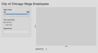
However once you select a department (e.g. City Council), the histrogram is correctly drawn. What gives? The problem is that if you do not select any values for selectInput(inputId = "department"), then the value of input$department is not all the possible values for employ$department – it’s value is NULL. So the employ data frame is being filtered to 0 rows because every observation has a value for department (even if that value is NA).
Fixing this is (relatively) simple. Inside the employ_filter reactive function, we should check if the department input exists, and if not then just not filter for that column. It’s easier to do this if we do not write employ_filter as a single piped operation:2
employ_filter <- reactive({
  employees <- employ

  # filter by department
  if(!is.null(input$department)) {
    employees <- filter(employees, department %in% input$department)
  }

  # filter by full or part-time
  employees <- filter(employees, full_time == input$full_time)

  # filter by hourly wage
  employees <- filter(employees,
                      wage >= input$wage[[1]],
                      wage <= input$wage[[2]])
})
Now when the render function tries to access input$department, it will get a NULL value before the user makes a selection and therefore skips filtering employ based on department. This also is a reliable fix if your app generates temporary error messages that vanish after a second. These may occur when the output relies on an object that has not yet been generated by the Shiny server() function.
Using uiOutput() to create UI elements dynamically
One of the output functions you can add in the UI is uiOutput(). According to the naming convention (e.g. plotOutput() is an output to render a plot), this is an output used to render more UI. This may sound a bit confusing, but it’s actually very useful. It’s usually used to create inputs (or any other UI) from the server, or in other words - you can create inputs dynamically.
Any input that you normally create in the UI is created when the app starts, and it cannot be changed. But what if one of your inputs depends on another input? In that case, you want to be able to create an input dynamically, in the server, and you would use uiOutput(). uiOutput() can be used to create any UI element, but it’s most often used to create input UI elements. The same rules regarding building outputs apply, which means the output (which is a UI element in this case) is created with the function renderUI().
Basic example of uiOutput()
As a very basic example, consider this app:
library(shiny)
ui <- fluidPage(
  numericInput("num", "Maximum slider value", 5),
  uiOutput("slider")
)

server <- function(input, output) {
  output$slider <- renderUI({
    sliderInput("slider", "Slider", min = 0,
                max = input$num, value = 0)
  })
}

shinyApp(ui = ui, server = server)
If you run that tiny app, you will see that whenever you change the value of the numeric input, the slider input is re-generated. This behavior can come in handy often.
Use uiOutput() in our app to populate the job titles
We can use this concept in our app to populate the choices for the job title selector. employ$job_title contains 145 distinct job titles, not all of which are applicable to every department. It would be helpful if we allow app users to filter the dataset by job title, we only allow as an input job titles which fall within the specified department(s).
First we need to add a placeholder for the selectInput() in the UI with:
uiOutput("jobTitle")
Then we need to create the output (which will create a UI element - yeah, it can be a bit confusing at first), so add the following code to the server function:
output$jobTitle <- renderUI({
  employees <- employ

  # filter by department
  if(!is.null(input$department)) {
    employees <- filter(employees, department %in% input$department)
  }

  # filter by full or part-time
  employees <- filter(employees, full_time == input$full_time)

  # filter by hourly wage
  employees <- filter(employees,
                      wage >= input$wage[[1]],
                      wage <= input$wage[[2]])

  selectInput(inputId = "jobTitle",
              label = "Job Title",
              choices = sort(unique(employees$job_title)),
              multiple = TRUE)
})
employ_filter() within this renderUI() function? Because we need to add a filter() in employ_filter() for the new job title selector. Relying on employ_filter() in output$jobTitle will generate a feedback loop preventing a user from reliably using the job title filter.Finally to make sure the data properly updates, change employ_filter in the server function to:
employ_filter <- reactive({
  employees <- employ

  # filter by department
  if(!is.null(input$department)) {
    employees <- filter(employees, department %in% input$department)
  }

  # filter by job title
  if(!is.null(input$jobTitle)) {
    employees <- filter(employees, job_title %in% input$jobTitle)
  }

  # filter by full or part-time
  employees <- filter(employees, full_time == input$full_time)

  # filter by hourly wage
  employees <- filter(employees,
                      wage >= input$wage[[1]],
                      wage <= input$wage[[2]])
})
Now if you run the app, you should be able to see the different job titles available for each department and the available job titles will update as you select specific departments.
Final Shiny app code
In case you got lost somewhere, here is the final code. The app is now functional, but there are plenty of features you can add to make it better.
library(shiny)
library(tidyverse)

employ <- read_csv("employees-wage.csv")

ui <- fluidPage(
  titlePanel("City of Chicago Wage Employees"),
  sidebarLayout(
    sidebarPanel(
      sliderInput(inputId = "wage",
                  label = "Wage range",
                  min = 0,
                  max = max(employ$wage, na.rm = TRUE),
                  value = c(0, max(employ$wage, na.rm = TRUE)),
                  pre = "$"),
      radioButtons(inputId = "full_time",
                   label = "Full or part-time",
                   choices = c("Full-Time", "Part-Time")),
      selectInput(inputId = "department",
                  label = "Department",
                  choices = sort(unique(employ$department)),
                  multiple = TRUE),
      uiOutput("jobTitle")
    ),
    mainPanel(plotOutput("hourlyPlot"),
              tableOutput("employTable"))
  )
)

server <- function(input, output) {
  employ_filter <- reactive({
    employees <- employ

    # filter by department
    if(!is.null(input$department)) {
      employees <- filter(employees, department %in% input$department)
    }

    # filter by job title
    if(!is.null(input$jobTitle)) {
      employees <- filter(employees, job_title %in% input$jobTitle)
    }

    # filter by full or part-time
    employees <- filter(employees, full_time == input$full_time)

    # filter by hourly wage
    employees <- filter(employees,
                        wage >= input$wage[[1]],
                        wage <= input$wage[[2]])
  })

  output$jobTitle <- renderUI({
    employees <- employ

    # filter by department
    if(!is.null(input$department)) {
      employees <- filter(employees, department %in% input$department)
    }

    # filter by full or part-time
    employees <- filter(employees, full_time == input$full_time)

    # filter by hourly wage
    employees <- filter(employees,
                        wage >= input$wage[[1]],
                        wage <= input$wage[[2]])

    selectInput(inputId = "jobTitle",
                label = "Job Title",
                choices = sort(unique(employees$job_title)),
                multiple = TRUE)
  })

  output$hourlyPlot <- renderPlot({
    ggplot(employ_filter(), aes(wage)) +
      geom_histogram()
  })

  output$employTable <- renderTable({
    employ_filter() %>%
      count(department)
  })
}

shinyApp(ui = ui, server = server)
Share your app with the world
Remember how every single app is a web page powered by an R session on a computer? So far, you’ve been running Shiny locally, which means your computer was used to power the app. It also means that the app was not accessible to anyone on the internet. If you want to share your app with the world, you need to host it somewhere.
Host on shinyapps.io
RStudio provides a service called shinyapps.io which lets you host your apps for free. It is integrated seamlessly into RStudio so that you can publish your apps with the click of a button, and it has a free version. The free version allows a certain number of apps per user and a certain number of activity on each app, but it should be good enough for most of you. It also lets you see some basic stats about usage of your app.
Hosting your app on shinyapps.io is the easy and recommended way of getting your app online. Go to www.shinyapps.io and sign up for an account. When you’re ready to publish your app, click on the “Publish Application” button in RStudio and follow their instructions. You might be asked to install a couple packages if it’s your first time.
After a successful deployment to shinyapps.io, you will be redirected to your app in the browser. You can use that URL to show off to your family what a cool app you wrote.
Host on a Shiny Server
The other option for hosting your app is on your own private Shiny server. Shiny Server is also a product by RStudio that lets you host apps on your own server. This means that instead of RStudio hosting the app for you, you have it on your own private server. This means you have a lot more freedom and flexibility, but it also means you need to have a server and be comfortable administering a server.
More Shiny features to check out
Shiny is extremely powerful and has lots of features that we haven’t covered. Here’s a sneak peek of just a few other common Shiny features that are not too advanced.
Shiny in Rmarkdown
You can include Shiny inputs and outputs in an Rmarkdown document! This means that your Rmarkdown document can be interactive. Learn more here. Here’s a simple example of how to include interactive Shiny elements in an R Markdown document:
---
output: html_document
runtime: shiny
---
`
``{r echo=FALSE, eval = TRUE}
sliderInput("num", "Choose a number",
0, 100, 20)
renderPlot({
plot(seq(input$num))
})
`
``
Use conditionalPanel() to conditionally show UI elements
You can use conditionalPanel() to either show or hide a UI element based on a simple condition, such as the value of another input. Learn more with ?conditionalPanel.
library(shiny)
ui <- fluidPage(
  numericInput("num", "Number", 5, 1, 10),
  conditionalPanel(
    "input.num >=5",
    "Hello!"
  )
)
server <- function(input, output) {}
shinyApp(ui = ui, server = server)
Use navbarPage() or tabsetPanel() to have multiple tabs in the UI
If your apps requires more than a single “view”, you can have separate tabs. Learn more with ?navbarPage or ?tabsetPanel.
library(shiny)
ui <- fluidPage(
  tabsetPanel(
    tabPanel("Tab 1", "Hello"),
    tabPanel("Tab 2", "there!")
  )
)
server <- function(input, output) {}
shinyApp(ui = ui, server = server)
Use DT for beautiful, interactive tables
Whenever you use tableOutput() + renderTable(), the table that Shiny creates is a static and boring-looking table. If you download the DT package, you can replace the default table with a much sleeker table by just using DT::dataTableOutput() + DT::renderDataTable(). It’s worth trying. Learn more on DT’s website.
Use isolate() function to remove a dependency on a reactive variable
When you have multiple reactive variables inside a reactive context, the whole code block will get re-executed whenever any of the reactive variables change because all the variables become dependencies of the code. If you want to suppress this behavior and cause a reactive variable to not be a dependency, you can wrap the code that uses that variable inside the isolate() function. Any reactive variables that are inside isolate() will not result in the code re-executing when their value is changed. Read more about this behavior with ?isolate.
Use update*Input() functions to update input values programmatically
Any input function has an equivalent update*Input function that can be used to update any of its parameters.
library(shiny)
ui <- fluidPage(
  sliderInput("slider", "Move me", value = 5, 1, 10),
  numericInput("num", "Number", value = 5, 1, 10)
)
server <- function(input, output, session) {
  observe({
    updateNumericInput(session, "num", value = input$slider)
  })
}
shinyApp(ui = ui, server = server)
Note that we used an additional argument session when defining the server function. While the input and output arguments are mandatory, the session argument is optional. You need to define the session argument when you want to use functions that need to access the session. The session parameter actually has some useful information in it, you can learn more about it with ?shiny::session.
Scoping rules in Shiny apps
Scoping is very important to understand in Shiny once you want to support more than one user at a time. Since your app can be hosted online, multiple users can use your app simultaneously. If there are any variables (such as datasets or global parameters) that should be shared by all users, then you can safely define them globally. But any variable that should be specific to each user’s session should be not be defined globally.
You can think of the server function as a sandbox for each user. Any code outside of the server function is run once and is shared by all the instances of your Shiny app. Any code inside the server is run once for every user that visits your app. This means that any user-specific variables should be defined inside server. If you look at the code in our Virginia ABC Store app, you’ll see that we followed this rule: the raw dataset was loaded outside the server and is therefore available to all users, but the employ_filter object is constructed inside the server so that every user has their own version of it. If employ_filter was a global variable, then when one user changes the values in your app, all other users connected to your app would see the change happen.
You can learn more about the scoping rules in Shiny here.
Use global.R to define objects available to both ui.R and server.R
If there are objects that you want to have available to both ui.R and server.R, you can place them in global.R. You can learn more about global.R and other scoping rules here.
Add images
You can add an image to your Shiny app by placing an image under the “www/” folder and using the UI function img(src = "image.png"). Shiny will know to automatically look in the “www/” folder for the image.
Add JavaScript/CSS
If you know JavaScript or CSS you are more than welcome to use some in your app.
library(shiny)
ui <- fluidPage(
  tags$head(tags$script("alert('Hello!');")),
  tags$head(tags$style("body{ color: blue; }")),
  "Hello"
)
server <- function(input, output) {

}
shinyApp(ui = ui, server = server)
If you do want to add some JavaScript or use common JavaScript functions in your apps, you might want to check out shinyjs.
Awesome add-on packages to Shiny
Many people have written packages that enhance Shiny in some way or add extra functionality. Here is a list of several popular packages that people often use together with Shiny:
shinyjs: Easily improve the user interaction and user experience in your Shiny apps in secondsshinythemes: Easily alter the appearance of your appleaflet: Add interactive maps to your appsggvis: Similar to ggplot2, but the plots are focused on being web-based and are more interactiveshinydashboard: Gives you tools to create visual “dashboards”
Resources
Shiny is a very popular package and has lots of resources on the web. Here’s a compiled list of a few resources which are all fairly easy to read and understand.
- Shiny official tutorial
- Shiny cheatsheet
- Lots of short useful articles about different topics in Shiny
- Shiny in Rmarkdown
- Get help from the Shiny Google group or StackOverflow
- Publish your apps for free with shinyapps.io
- Learn about how reactivity works
- Learn about useful debugging techniques
- Shiny tips & tricks for improving your apps and solving common problems
Acknowledgments
- This page is derived in part from “UBC STAT 545A and 547M”, licensed under the CC BY-NC 3.0 Creative Commons License.
Session Info
sessioninfo::session_info()
## ─ Session info ───────────────────────────────────────────────────────────────
##  setting  value
##  version  R version 4.2.1 (2022-06-23)
##  os       macOS Monterey 12.3
##  system   aarch64, darwin20
##  ui       X11
##  language (EN)
##  collate  en_US.UTF-8
##  ctype    en_US.UTF-8
##  tz       America/New_York
##  date     2022-08-22
##  pandoc   2.18 @ /Applications/RStudio.app/Contents/MacOS/quarto/bin/tools/ (via rmarkdown)
##
## ─ Packages ───────────────────────────────────────────────────────────────────
##  package       * version    date (UTC) lib source
##  assertthat      0.2.1      2019-03-21 [2] CRAN (R 4.2.0)
##  backports       1.4.1      2021-12-13 [2] CRAN (R 4.2.0)
##  blogdown        1.10       2022-05-10 [2] CRAN (R 4.2.0)
##  bookdown        0.27       2022-06-14 [2] CRAN (R 4.2.0)
##  broom           1.0.0      2022-07-01 [2] CRAN (R 4.2.0)
##  bslib           0.4.0      2022-07-16 [2] CRAN (R 4.2.0)
##  cachem          1.0.6      2021-08-19 [2] CRAN (R 4.2.0)
##  cellranger      1.1.0      2016-07-27 [2] CRAN (R 4.2.0)
##  cli             3.3.0      2022-04-25 [2] CRAN (R 4.2.0)
##  colorspace      2.0-3      2022-02-21 [2] CRAN (R 4.2.0)
##  crayon          1.5.1      2022-03-26 [2] CRAN (R 4.2.0)
##  DBI             1.1.3      2022-06-18 [2] CRAN (R 4.2.0)
##  dbplyr          2.2.1      2022-06-27 [2] CRAN (R 4.2.0)
##  digest          0.6.29     2021-12-01 [2] CRAN (R 4.2.0)
##  dplyr         * 1.0.9      2022-04-28 [2] CRAN (R 4.2.0)
##  ellipsis        0.3.2      2021-04-29 [2] CRAN (R 4.2.0)
##  evaluate        0.16       2022-08-09 [1] CRAN (R 4.2.1)
##  fansi           1.0.3      2022-03-24 [2] CRAN (R 4.2.0)
##  fastmap         1.1.0      2021-01-25 [2] CRAN (R 4.2.0)
##  forcats       * 0.5.1      2021-01-27 [2] CRAN (R 4.2.0)
##  fs              1.5.2      2021-12-08 [2] CRAN (R 4.2.0)
##  gargle          1.2.0      2021-07-02 [2] CRAN (R 4.2.0)
##  generics        0.1.3      2022-07-05 [2] CRAN (R 4.2.0)
##  ggplot2       * 3.3.6      2022-05-03 [2] CRAN (R 4.2.0)
##  glue            1.6.2      2022-02-24 [2] CRAN (R 4.2.0)
##  googledrive     2.0.0      2021-07-08 [2] CRAN (R 4.2.0)
##  googlesheets4   1.0.0      2021-07-21 [2] CRAN (R 4.2.0)
##  gtable          0.3.0      2019-03-25 [2] CRAN (R 4.2.0)
##  haven           2.5.0      2022-04-15 [2] CRAN (R 4.2.0)
##  here            1.0.1      2020-12-13 [2] CRAN (R 4.2.0)
##  hms             1.1.1      2021-09-26 [2] CRAN (R 4.2.0)
##  htmltools       0.5.3      2022-07-18 [2] CRAN (R 4.2.0)
##  httpuv          1.6.5      2022-01-05 [2] CRAN (R 4.2.0)
##  httr            1.4.3      2022-05-04 [2] CRAN (R 4.2.0)
##  jquerylib       0.1.4      2021-04-26 [2] CRAN (R 4.2.0)
##  jsonlite        1.8.0      2022-02-22 [2] CRAN (R 4.2.0)
##  knitr           1.39       2022-04-26 [2] CRAN (R 4.2.0)
##  later           1.3.0      2021-08-18 [2] CRAN (R 4.2.0)
##  lifecycle       1.0.1      2021-09-24 [2] CRAN (R 4.2.0)
##  lubridate       1.8.0      2021-10-07 [2] CRAN (R 4.2.0)
##  magrittr        2.0.3      2022-03-30 [2] CRAN (R 4.2.0)
##  mime            0.12       2021-09-28 [2] CRAN (R 4.2.0)
##  modelr          0.1.8      2020-05-19 [2] CRAN (R 4.2.0)
##  munsell         0.5.0      2018-06-12 [2] CRAN (R 4.2.0)
##  pillar          1.8.0      2022-07-18 [2] CRAN (R 4.2.0)
##  pkgconfig       2.0.3      2019-09-22 [2] CRAN (R 4.2.0)
##  promises        1.2.0.1    2021-02-11 [2] CRAN (R 4.2.0)
##  purrr         * 0.3.4      2020-04-17 [2] CRAN (R 4.2.0)
##  R6              2.5.1      2021-08-19 [2] CRAN (R 4.2.0)
##  Rcpp            1.0.9      2022-07-08 [2] CRAN (R 4.2.0)
##  readr         * 2.1.2      2022-01-30 [2] CRAN (R 4.2.0)
##  readxl          1.4.0      2022-03-28 [2] CRAN (R 4.2.0)
##  reprex          2.0.1.9000 2022-08-10 [1] Github (tidyverse/reprex@6d3ad07)
##  rlang           1.0.4      2022-07-12 [2] CRAN (R 4.2.0)
##  rmarkdown       2.14       2022-04-25 [2] CRAN (R 4.2.0)
##  rprojroot       2.0.3      2022-04-02 [2] CRAN (R 4.2.0)
##  rstudioapi      0.13       2020-11-12 [2] CRAN (R 4.2.0)
##  rvest           1.0.2      2021-10-16 [2] CRAN (R 4.2.0)
##  sass            0.4.2      2022-07-16 [2] CRAN (R 4.2.0)
##  scales          1.2.0      2022-04-13 [2] CRAN (R 4.2.0)
##  sessioninfo     1.2.2      2021-12-06 [2] CRAN (R 4.2.0)
##  shiny         * 1.7.2      2022-07-19 [2] CRAN (R 4.2.0)
##  stringi         1.7.8      2022-07-11 [2] CRAN (R 4.2.0)
##  stringr       * 1.4.0      2019-02-10 [2] CRAN (R 4.2.0)
##  tibble        * 3.1.8      2022-07-22 [2] CRAN (R 4.2.0)
##  tidyr         * 1.2.0      2022-02-01 [2] CRAN (R 4.2.0)
##  tidyselect      1.1.2      2022-02-21 [2] CRAN (R 4.2.0)
##  tidyverse     * 1.3.2      2022-07-18 [2] CRAN (R 4.2.0)
##  tzdb            0.3.0      2022-03-28 [2] CRAN (R 4.2.0)
##  utf8            1.2.2      2021-07-24 [2] CRAN (R 4.2.0)
##  vctrs           0.4.1      2022-04-13 [2] CRAN (R 4.2.0)
##  withr           2.5.0      2022-03-03 [2] CRAN (R 4.2.0)
##  xfun            0.31       2022-05-10 [1] CRAN (R 4.2.0)
##  xml2            1.3.3      2021-11-30 [2] CRAN (R 4.2.0)
##  xtable          1.8-4      2019-04-21 [2] CRAN (R 4.2.0)
##  yaml            2.3.5      2022-02-21 [2] CRAN (R 4.2.0)
##
##  [1] /Users/soltoffbc/Library/R/arm64/4.2/library
##  [2] /Library/Frameworks/R.framework/Versions/4.2-arm64/Resources/library
##
## ──────────────────────────────────────────────────────────────────────────────
Feel free to explore the full employee dataset for homework 11, but we will only focus on the wage employees today because there are different variables relevant to wage vs. salaried employees. We don’t want to get into that confusion today. ↩︎
But it is possible. ↩︎