Bugs and styling code
library(tidyverse)
set.seed(1234)
Run the code below in your console to download this exercise as a set of R scripts.
usethis::use_course("cis-ds/debugging-and-defensive-programming")
A software bug is “an error, flaw, failure or fault in a computer program or system that causes it to produce an incorrect or unexpected result, or to behave in unintended ways.”1 In an ideal world, the computer will warn you when it encounters a bug. R has the ability to do this in some situations (see our discussion below of errors, warnings, and messages). However bugs also arise because you expect the program to do one thing but provide it the ability to perform different from expectations.
As I have repeatedly emphasized in class, computers are powerful tools that are incredibly stupid. They will do exactly what you tell them to, nothing more and nothing less. If you write your code in a way that allows it to behave in an unintended way, this is your fault. The first goal of debugging should be to prevent unintended behaviors before they strike. However, when such bugs occur we need the tools and knowledge to track down these unintended behaviors and correct them in our code.
The most important step to debugging is to prevent bugs in the first place. There are several methods we can employ to do that. Some of them are simple such as styling our code so that we follow consistent practices when writing scripts and programs. Consistency will prevent silly and minor mistakes such as typos. Good styles also make our code more readable for the human eye and allow us to isolate and detect errors merely by looking at the screen. Others are more advanced and focus on the concept of failing fast - as soon as something goes wrong, stop executing the program and announce an error.
Writing code
Think back to the analogy of programming languages to human languages. Programming languages adhere to a specific grammar and syntax, they contain a vocabulary, etymology, cultural conventions, word roots (prefixes and suffixes), just like English or any other written or spoken language. We can therefore equate different components of a program to their language counterparts:
| Programming | Language |
|---|---|
| Scripts | Essays |
| Sections | Paragraphs |
| Lines Breaks | Sentences |
| Parentheses | Punctuation |
| Functions | Verbs |
| Variables | Nouns |
Now think about how you write a document in English. In 1987, the Challenger space shuttle exploded just 73 seconds after takeoff. The deaths of seven crewmembers were seen live by millions of American schoolchildren watching around the country. A few hours after the tragedy, President Ronald Reagan gave a national address.
Here is an excerpt of that address:
weve grown used to wonders in this century its hard to dazzle us but for 25 years the united states space program has been doing just that weve grown used to the idea of space and perhaps we forget that weve only just begun were still pioneers they the members of the Challenger crew were pioneers and i want to say something to the school children of America who were watching the live coverage of the shuttles takeoff i know it is hard to understand but sometimes painful things like this happen its all part of the process of exploration and discovery its all part of taking a chance and expanding mans horizons the future doesnt belong to the fainthearted it belongs to the brave the challenger crew was pulling us into the future and well continue to follow them the crew of the space shuttle challenger honored us by the manner in which they lived their lives we will never forget them nor the last time we saw them this morning as they prepared for the journey and waved goodbye and slipped the surly bonds of earth to touch the face of god
Wait a minute, this doesn’t look right. What happened to the punctuation? The capitalization? Where are all the sentences and paragraph breaks? Isn’t this hard to read and understand? Do you feel any of the emotions of the moment? Probably not, because the normal rules of grammar and syntax have been destroyed. Here’s the same excerpt, but properly styled:
We’ve grown used to wonders in this century. It’s hard to dazzle us. But for 25 years the United States space program has been doing just that. We’ve grown used to the idea of space, and perhaps we forget that we’ve only just begun. We’re still pioneers. They, the members of the Challenger crew, were pioneers.
And I want to say something to the school children of America who were watching the live coverage of the shuttle’s takeoff. I know it is hard to understand, but sometimes painful things like this happen. It’s all part of the process of exploration and discovery. It’s all part of taking a chance and expanding man’s horizons. The future doesn’t belong to the fainthearted; it belongs to the brave. The Challenger crew was pulling us into the future, and we’ll continue to follow them….
The crew of the space shuttle Challenger honoured us by the manner in which they lived their lives. We will never forget them, nor the last time we saw them, this morning, as they prepared for the journey and waved goodbye and ‘slipped the surly bonds of earth’ to ’touch the face of God.’
That makes much more sense. Adhering to standard rules of style make the text more legible and interpretable. This is what we should aim for when writing programs in R.2
Style guide
Here are some common rules you should adopt when writing code in R, adapted from Hadley Wickham’s style guide.
Notation and naming
File names
Files should have intuitive and meaningful names. Avoid spaces or non-standard characters in your file names. R scripts should always end in .R; R Markdown documents should always end in .Rmd.
# Good
fit-models.R
utility-functions.R
gun-deaths.Rmd

# Bad
foo.r
stuff.r
gun deaths.rmd
Object names
Variables refer to data objects such as vectors, lists, or data frames. Variable and function names should be lowercase. Use an underscore (_) to separate words within a name. Avoid using periods (.).3 Variable names should generally be nouns and function names should be verbs. Try to pick names that are concise and meaningful.
# Good
day_one
day_1

# Bad
first_day_of_the_month
DayOne
dayone
djm1
Where possible, avoid using names of existing functions and variables. Doing so will cause confusion for the readers of your code, not to mention make it difficult to access the existing functions and variables.
# Bad
T <- FALSE
c <- 10
For instance, what would happen if I created a new mean() function?
x <- seq(from = 1, to = 10)
mean(x)
## [1] 5.5
# create new mean function
mean <- function(x) sum(x)
mean(x)
[1] 55

Syntax
Spacing
Place spaces around all infix operators (=, +, -, <-, etc.). The same rule applies when using = in function calls.
# Good
average <- mean(feet / 12 + inches, na.rm = TRUE)

# Bad
average<-mean(feet/12+inches,na.rm=TRUE)
Place a space before left parentheses, except in a function call.
if-else or for loops. I typically never place a space before left parentheses, but it is supposed to be good practice. Just remember to be consistent whatever approach you choose.# Good
if (debug) do(x)
plot(x, y)
# Bad
if(debug)do(x)
plot (x, y)
Do not place spaces around code in parentheses or square brackets (unless there’s a comma, in which case see above).
# Good
if (debug) do(x)
penguins[5, ]

# Bad
if ( debug ) do(x)  # No spaces around debug
x[1,]   # Needs a space after the comma
x[1 ,]  # Space goes after comma not before
Curly braces
An opening curly brace should never go on its own line and should always be followed by a new line. A closing curly brace should always go on its own line, unless it’s followed by else.
Always indent the code inside curly braces.
# Good

if (y < 0 && debug) {
  message("Y is negative")
}

if (y == 0) {
  log(x)
} else {
  y ^ x
}

# Bad

if (y < 0 && debug)
message("Y is negative")

if (y == 0) {
log(x)
} else { y ^ x }
It’s ok to leave very short statements on the same line:
if (y < 0 && debug) message("Y is negative")
Line length
Strive to limit your code to 80 characters per line. This fits comfortably on a printed page with a reasonably sized font. For instance, if I wanted to convert the chief column to a factor for building a faceted graph:
# Good
scdbv <- mutate(scdbv,
                chief = factor(chief, levels = c("Jay", "Rutledge", "Ellsworth",
                                                 "Marshall", "Taney", "Chase",
                                                 "Waite", "Fuller", "White",
                                                 "Taft", "Hughes", "Stone",
                                                 "Vinson", "Warren", "Burger",
                                                 "Rehnquist", "Roberts")))

# Bad
scdbv <- mutate(scdbv, chief = factor(chief, levels = c("Jay", "Rutledge", "Ellsworth", "Marshall", "Taney", "Chase", "Waite", "Fuller", "White", "Taft", "Hughes", "Stone", "Vinson", "Warren", "Burger", "Rehnquist", "Roberts")))
Indentation
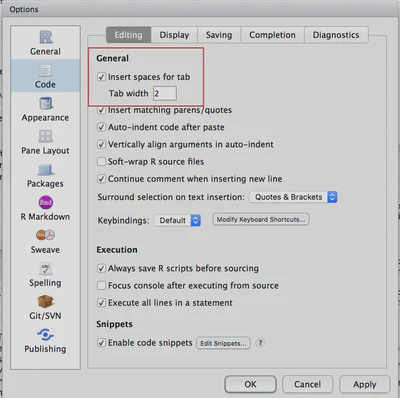
When indenting your code, use two spaces. Never use tabs or mix tabs and spaces.
The only exception is if a function definition runs over multiple lines. In that case, indent the second line to where the definition starts:
# pure function
long_function_name <- function(a = "a long argument",
                               b = "another argument",
                               c = "another long argument") {
  # As usual code is indented by two spaces.
}

# in a mutate() function
scdbv <- scdbv %>%
  mutate(majority = majority - 1,
         chief = factor(chief, levels = c("Jay", "Rutledge", "Ellsworth",
                                          "Marshall", "Taney", "Chase",
                                          "Waite", "Fuller", "White",
                                          "Taft", "Hughes", "Stone",
                                          "Vinson", "Warren", "Burger",
                                          "Rehnquist", "Roberts")))
Assignment
Use <-, not =, for assignment. Why? Because I said so. Or read more here.
# Good
x <- 5
# Bad
x = 5
Calling functions
If a package is loaded using library(), you can directly access functions by referring to the function name. For example, if you want to use the map() function from the purrr package, you could do the following:
library(purrr)
map()
Sometimes different packages use the same name for very different functions. Here, map() from the purrr package performs iterative operations. However map() from the maps package allows you to draw maps in R.
By default, if you load packages with functions that share the same name, a direct reference to the function will use the most recently loaded package. So in this code chunk
library(purrr)
library(maps)

map()
You would be using map() from the maps package. To use a function from a specific library, use :: notation, like this:
library(purrr)
library(maps)

purrr::map()    # use map() from the purrr library
maps::map()     # use map() from the maps library
You can also use this notation to access a function from a library that has not been loaded into your R session:
library(purrr)

map()           # use map() from the purrr library
maps::map()     # use map() from the maps library
Comments
Comment your code. Each line of a comment should begin with the comment symbol and a single space: #. Comments should explain the why, not the what.
To take advantage of RStudio’s code folding feature, add at least four trailing dashes (-), equal signs (=), or pound signs (#) after the comment text
# Section One ---------------------------------

# Section Two =================================

### Section Three #############################
Auto-formatting in RStudio
There are two built-in methods of using RStudio to automatically format and clean up your code. They are not perfect, but can help in some circumstances.
Format code
Code > Reformat Code (Shift + Cmd/Ctrl + A)
Bad code
# comments are retained
1+1

if(TRUE){
x=1  # inline comments
}else{
x=2;print('Oh no... ask the right bracket to go away!')}
1*3 # one space before this comment will become two!
2+2+2    # only 'single quotes' are allowed in comments

penguins %>%
filter(island == "Torgersen") %>%
group_by(species) %>%
summarize(body_mass = mean(body_mass_g, na.rm = TRUE))

lm(y~x1+x2, data=data.frame(y=rnorm(100),x1=rnorm(100),x2=rnorm(100)))  ### a linear model

1+1+1+1+1+1+1+1+1+1+1+1+1+1+1+1+1+1+1+1+1+1+1  ## comments after a long line
## here is a long long long long long long long long long long long long long long long long long long long comment
Better code
# comments are retained
1 + 1

if (TRUE) {
  x <- 1 # inline comments
} else {
  x <- 2
  print("Oh no... ask the right bracket to go away!")
}
1 * 3 # one space before this comment will become two!
2 + 2 + 2 # only 'single quotes' are allowed in comments

penguins %>%
  filter(island == "Torgersen") %>%
  group_by(species) %>%
  summarize(body_mass = mean(body_mass_g, na.rm = TRUE))

lm(y ~ x1 + x2, data = data.frame(
  y = rnorm(100),
  x1 = rnorm(100),
  x2 = rnorm(100)
)) ### a linear model

1 + 1 + 1 + 1 + 1 + 1 + 1 + 1 + 1 + 1 + 1 + 1 + 1 + 1 + 1 + 1 + 1 + 1 +
  1 + 1 + 1 + 1 + 1 ## comments after a long line
## here is a long long long long long long long long long long long long long long long long long long long comment
Format code will attempt to adjust the source code formatting to adhere to the style guide specified above. It doesn’t look perfect, but is more readable than the original. We should still clean up some of this manually, such as the comment on the last line that flows over.
Reindent lines
Code > Reindent Lines (Cmd/Ctrl + I)
Bad code
# comments are retained
1 + 1

if (TRUE) {
x = 1  # inline comments
} else{
x = 2
print('Oh no... ask the right bracket to go away!')
}
1 * 3 # one space before this comment will become two!
2 + 2 + 2    # only 'single quotes' are allowed in comments

penguins %>%
filter(island == "Torgersen") %>%
group_by(species) %>%
summarize(body_mass = mean(body_mass_g, na.rm = TRUE))

lm(y ~ x1 + x2, data = data.frame(
y = rnorm(100),
x1 = rnorm(100),
x2 = rnorm(100)
))  ### a linear model

1 + 1 + 1 + 1 + 1 + 1 + 1 + 1 + 1 + 1 + 1 + 1 + 1 + 1 + 1 + 1 + 1 + 1 +
1 + 1 + 1 + 1 + 1  ## comments after a long line
## here is a long long long long long long long long long long long long long long long long long long long comment
Better code
# comments are retained
1 + 1

if (TRUE) {
  x <- 1 # inline comments
} else {
  x <- 2
  print("Oh no... ask the right bracket to go away!")
}
1 * 3 # one space before this comment will become two!
2 + 2 + 2 # only 'single quotes' are allowed in comments

penguins %>%
  filter(island == "Torgersen") %>%
  group_by(species) %>%
  summarize(body_mass = mean(body_mass_g, na.rm = TRUE))

lm(y ~ x1 + x2, data = data.frame(
  y = rnorm(100),
  x1 = rnorm(100),
  x2 = rnorm(100)
)) ### a linear model

1 + 1 + 1 + 1 + 1 + 1 + 1 + 1 + 1 + 1 + 1 + 1 + 1 + 1 + 1 + 1 + 1 + 1 +
  1 + 1 + 1 + 1 + 1 ## comments after a long line
## here is a long long long long long long long long long long long long long long long long long long long comment
Reindent lines will add spacing to conditional expression blocks, multi-line functions, expressions which run over multiple lines, and piped operations. Again, it is not perfect but it does some of the formatting work for us.
styler
styler is a package that auto-formats R source code to adhere to the tidyverse formatting rules. You can re-style a snippet of code, an entire .R/.Rmd file, or a directory of .R/.Rmd files.
See the introduction for examples of how to re-format code using this package.
Exercise: style this code
Here’s a chunk of code from an exercise from a different class. It is formatted terribly, but as you can see it does work - the computer can interpret it. Use the style guide to clean it up and make it readable.
library(tidyverse)
library(modelr)
library(broom)
library(gam)
College <- as_tibble(ISLR::College) %>%
mutate(Outstate = Outstate / 1000,
Room.Board = Room.Board / 1000,
PhD_log = log(PhD)) # rescale Outstate in thousands of dollars
crossv_kfold(College, k = 10) %>%
mutate(linear = map(train, ~ glm(Outstate ~ PhD,
data = .)),
log = map(train, ~ glm(Outstate ~ PhD_log, data = .)),
spline = map(train, ~ glm(Outstate ~ bs(PhD, df = 5), data = .))) %>% gather(type, model, linear:spline) %>%
mutate(mse = map2_dbl(model, test, mse)) %>% group_by(type) %>%
summarize(mse = mean(mse)) # k-fold cv of three model types
college_phd_spline <- gam(Outstate ~ bs(PhD, df = 5), data = College) # spline has the best model fit
college_phd_terms <- preplot(college_phd_spline, se = TRUE, rug = FALSE) # get first difference for age
# age plot
tibble(
x = college_phd_terms$`bs(PhD, df = 5)`$x,
y = college_phd_terms$`bs(PhD, df = 5)`$y,
se.fit = college_phd_terms$`bs(PhD, df = 5)`$se.y
)%>%mutate(y_low = y - 1.96 * se.fit, y_high = y + 1.96 * se.fit) %>%
ggplot(aes(x, y))+geom_line()+
geom_line(aes(y = y_low), linetype = 2)+
geom_line(aes(y = y_high), linetype = 2) +
labs(title = "Cubic spline of out-of-state tuition",
subtitle = "Knots = 2",
x = "Percent of faculty with PhDs", y = expression(f[1](PhD)))
Click for the solution
library(tidyverse)
library(modelr)
library(broom)
library(gam)

# rescale Outstate in thousands of dollars
College <- as_tibble(ISLR::College) %>%
  mutate(
    Outstate = Outstate / 1000,
    Room.Board = Room.Board / 1000,
    PhD_log = log(PhD)
  )

# k-fold cv of three model types
crossv_kfold(College, k = 10) %>%
  mutate(
    linear = map(train, ~ glm(Outstate ~ PhD,
      data = .
    )),
    log = map(train, ~ glm(Outstate ~ PhD_log, data = .)),
    spline = map(train, ~ glm(Outstate ~ bs(PhD, df = 5), data = .))
  ) %>%
  gather(type, model, linear:spline) %>%
  mutate(mse = map2_dbl(model, test, mse)) %>%
  group_by(type) %>%
  summarize(mse = mean(mse))

# spline has the best model fit
college_phd_spline <- gam(Outstate ~ bs(PhD, df = 5), data = College)

# get first difference for age
college_phd_terms <- preplot(college_phd_spline, se = TRUE, rug = FALSE)

# age plot
tibble(
  x = college_phd_terms$`bs(PhD, df = 5)`$x,
  y = college_phd_terms$`bs(PhD, df = 5)`$y,
  se.fit = college_phd_terms$`bs(PhD, df = 5)`$se.y
) %>%
  mutate(y_low = y - 1.96 * se.fit, y_high = y + 1.96 * se.fit) %>%
  ggplot(aes(x, y)) +
  geom_line() +
  geom_line(aes(y = y_low), linetype = 2) +
  geom_line(aes(y = y_high), linetype = 2) +
  labs(
    title = "Cubic spline of out-of-state tuition",
    subtitle = "Knots = 2",
    x = "Percent of faculty with PhDs",
    y = expression(f[1](PhD))
  )
Session Info
sessioninfo::session_info()
## ─ Session info ───────────────────────────────────────────────────────────────
##  setting  value
##  version  R version 4.2.1 (2022-06-23)
##  os       macOS Monterey 12.3
##  system   aarch64, darwin20
##  ui       X11
##  language (EN)
##  collate  en_US.UTF-8
##  ctype    en_US.UTF-8
##  tz       America/New_York
##  date     2022-08-22
##  pandoc   2.18 @ /Applications/RStudio.app/Contents/MacOS/quarto/bin/tools/ (via rmarkdown)
##
## ─ Packages ───────────────────────────────────────────────────────────────────
##  package       * version    date (UTC) lib source
##  assertthat      0.2.1      2019-03-21 [2] CRAN (R 4.2.0)
##  backports       1.4.1      2021-12-13 [2] CRAN (R 4.2.0)
##  blogdown        1.10       2022-05-10 [2] CRAN (R 4.2.0)
##  bookdown        0.27       2022-06-14 [2] CRAN (R 4.2.0)
##  broom           1.0.0      2022-07-01 [2] CRAN (R 4.2.0)
##  bslib           0.4.0      2022-07-16 [2] CRAN (R 4.2.0)
##  cachem          1.0.6      2021-08-19 [2] CRAN (R 4.2.0)
##  cellranger      1.1.0      2016-07-27 [2] CRAN (R 4.2.0)
##  cli             3.3.0      2022-04-25 [2] CRAN (R 4.2.0)
##  colorspace      2.0-3      2022-02-21 [2] CRAN (R 4.2.0)
##  crayon          1.5.1      2022-03-26 [2] CRAN (R 4.2.0)
##  DBI             1.1.3      2022-06-18 [2] CRAN (R 4.2.0)
##  dbplyr          2.2.1      2022-06-27 [2] CRAN (R 4.2.0)
##  digest          0.6.29     2021-12-01 [2] CRAN (R 4.2.0)
##  dplyr         * 1.0.9      2022-04-28 [2] CRAN (R 4.2.0)
##  ellipsis        0.3.2      2021-04-29 [2] CRAN (R 4.2.0)
##  evaluate        0.16       2022-08-09 [1] CRAN (R 4.2.1)
##  fansi           1.0.3      2022-03-24 [2] CRAN (R 4.2.0)
##  fastmap         1.1.0      2021-01-25 [2] CRAN (R 4.2.0)
##  forcats       * 0.5.1      2021-01-27 [2] CRAN (R 4.2.0)
##  fs              1.5.2      2021-12-08 [2] CRAN (R 4.2.0)
##  gargle          1.2.0      2021-07-02 [2] CRAN (R 4.2.0)
##  generics        0.1.3      2022-07-05 [2] CRAN (R 4.2.0)
##  ggplot2       * 3.3.6      2022-05-03 [2] CRAN (R 4.2.0)
##  glue            1.6.2      2022-02-24 [2] CRAN (R 4.2.0)
##  googledrive     2.0.0      2021-07-08 [2] CRAN (R 4.2.0)
##  googlesheets4   1.0.0      2021-07-21 [2] CRAN (R 4.2.0)
##  gtable          0.3.0      2019-03-25 [2] CRAN (R 4.2.0)
##  haven           2.5.0      2022-04-15 [2] CRAN (R 4.2.0)
##  here            1.0.1      2020-12-13 [2] CRAN (R 4.2.0)
##  hms             1.1.1      2021-09-26 [2] CRAN (R 4.2.0)
##  htmltools       0.5.3      2022-07-18 [2] CRAN (R 4.2.0)
##  httr            1.4.3      2022-05-04 [2] CRAN (R 4.2.0)
##  jquerylib       0.1.4      2021-04-26 [2] CRAN (R 4.2.0)
##  jsonlite        1.8.0      2022-02-22 [2] CRAN (R 4.2.0)
##  knitr           1.39       2022-04-26 [2] CRAN (R 4.2.0)
##  lifecycle       1.0.1      2021-09-24 [2] CRAN (R 4.2.0)
##  lubridate       1.8.0      2021-10-07 [2] CRAN (R 4.2.0)
##  magrittr        2.0.3      2022-03-30 [2] CRAN (R 4.2.0)
##  modelr          0.1.8      2020-05-19 [2] CRAN (R 4.2.0)
##  munsell         0.5.0      2018-06-12 [2] CRAN (R 4.2.0)
##  pillar          1.8.0      2022-07-18 [2] CRAN (R 4.2.0)
##  pkgconfig       2.0.3      2019-09-22 [2] CRAN (R 4.2.0)
##  purrr         * 0.3.4      2020-04-17 [2] CRAN (R 4.2.0)
##  R6              2.5.1      2021-08-19 [2] CRAN (R 4.2.0)
##  readr         * 2.1.2      2022-01-30 [2] CRAN (R 4.2.0)
##  readxl          1.4.0      2022-03-28 [2] CRAN (R 4.2.0)
##  reprex          2.0.1.9000 2022-08-10 [1] Github (tidyverse/reprex@6d3ad07)
##  rlang           1.0.4      2022-07-12 [2] CRAN (R 4.2.0)
##  rmarkdown       2.14       2022-04-25 [2] CRAN (R 4.2.0)
##  rprojroot       2.0.3      2022-04-02 [2] CRAN (R 4.2.0)
##  rstudioapi      0.13       2020-11-12 [2] CRAN (R 4.2.0)
##  rvest           1.0.2      2021-10-16 [2] CRAN (R 4.2.0)
##  sass            0.4.2      2022-07-16 [2] CRAN (R 4.2.0)
##  scales          1.2.0      2022-04-13 [2] CRAN (R 4.2.0)
##  sessioninfo     1.2.2      2021-12-06 [2] CRAN (R 4.2.0)
##  stringi         1.7.8      2022-07-11 [2] CRAN (R 4.2.0)
##  stringr       * 1.4.0      2019-02-10 [2] CRAN (R 4.2.0)
##  tibble        * 3.1.8      2022-07-22 [2] CRAN (R 4.2.0)
##  tidyr         * 1.2.0      2022-02-01 [2] CRAN (R 4.2.0)
##  tidyselect      1.1.2      2022-02-21 [2] CRAN (R 4.2.0)
##  tidyverse     * 1.3.2      2022-07-18 [2] CRAN (R 4.2.0)
##  tzdb            0.3.0      2022-03-28 [2] CRAN (R 4.2.0)
##  utf8            1.2.2      2021-07-24 [2] CRAN (R 4.2.0)
##  vctrs           0.4.1      2022-04-13 [2] CRAN (R 4.2.0)
##  withr           2.5.0      2022-03-03 [2] CRAN (R 4.2.0)
##  xfun            0.31       2022-05-10 [1] CRAN (R 4.2.0)
##  xml2            1.3.3      2021-11-30 [2] CRAN (R 4.2.0)
##  yaml            2.3.5      2022-02-21 [2] CRAN (R 4.2.0)
##
##  [1] /Users/soltoffbc/Library/R/arm64/4.2/library
##  [2] /Library/Frameworks/R.framework/Versions/4.2-arm64/Resources/library
##
## ──────────────────────────────────────────────────────────────────────────────
And for that matter, in any other programming language as well. Note however that these style rules are specific to R; other languages by necessity may use different rules and conventions. ↩︎
These are useful for writing functions for generic methods. ↩︎