Iteration
library(tidyverse)
library(rcis)
library(palmerpenguins)
library(modeldata)

set.seed(1234)
theme_set(theme_minimal())
Run the code below in your console to download this exercise as a set of R scripts.
usethis::use_course("cis-ds/vectors-and-iteration")
Writing for loops
Functions are one method of reducing duplication in your code. Another tool for reducing duplication is iteration, which lets you do the same thing to multiple inputs.
Example for loop
df <- tibble(
  a = rnorm(10),
  b = rnorm(10),
  c = rnorm(10),
  d = rnorm(10)
)
Let’s say we want to compute the median for each column.
median(df$a)
## [1] -0.5555419
median(df$b)
## [1] -0.4941011
median(df$c)
## [1] -0.4656169
median(df$d)
## [1] -0.605349
Boo! We’ve copied-and-pasted median() three times. We don’t want to do that. Instead, we can use a for loop:
output <- vector(mode = "double", length = ncol(df))
for (i in seq_along(df)) {
  output[[i]] <- median(df[[i]])
}
output
## [1] -0.5555419 -0.4941011 -0.4656169 -0.6053490
Let’s review the three components of every for loop.
Output
output <- vector("double", length = ncol(df))
Before you start a loop, you need to create an empty vector to store the output of the loop. Preallocating space for your output is much more efficient than creating space as you move through the loop. The vector() function allows you to create an empty vector of any type. The first argument mode defines the type of vector (“logical”, “integer”, “double”, “character”, etc.) and the second argument length defines the length of the vector.
Numeric vectors are initialized to 0, logical vectors are initialized to FALSE, character vectors are initialized to "", and list elements to NULL.
vector(mode = "double", length = ncol(df))
## [1] 0 0 0 0
vector(mode = "logical", length = ncol(df))
## [1] FALSE FALSE FALSE FALSE
vector(mode = "character", length = ncol(df))
## [1] "" "" "" ""
vector(mode = "list", length = ncol(df))
## [[1]]
## NULL
##
## [[2]]
## NULL
##
## [[3]]
## NULL
##
## [[4]]
## NULL
Sequence
i in seq_along(df)
This component determines what to loop over. During each iteration through the for loop, a new value will be assigned to i based on the the defined sequence. Here, the sequence is seq_along(df) which creates a numeric vector for a sequence of numbers beginning at 1 and continuing until it reaches the length of df (the length here is the number of columns in df).
seq_along(df)
## [1] 1 2 3 4
Body
output[[i]] <- median(df[[i]])
This is the code that actually performs the desired calculations. It runs multiple times for every value of i. We use [[ notation to reference each column of df and store it in the appropriate element in output.
Why we preallocate space for the output
If you don’t preallocate space for the output, each time the for loop iterates, it makes a copy of the output and appends the new value at the end. Copying data takes time and memory. If the output is preallocated space, the loop simply fills in the slots with the correct values.
Consider the following task: duplicate the data frame palmerpenguins::penguins 100 times and bind them together into a single data frame. We can accomplish the latter task using bind_rows(), and use a for loop to create 100 copies of penguins. What is the difference if we preallocate space for the output as opposed to just copying and extending the data frame each time?
# no preallocation
penguins_no_preall <- tibble()

for(i in 1:100){
  penguins_no_preall <- bind_rows(penguins_no_preall, penguins)
}

# with preallocation using a list
penguins_preall <- vector(mode = "list", length = 100)

for(i in 1:100){
  penguins_preall[[i]] <- penguins
}

penguins_preall <- bind_rows(penguins_preall)
Let’s compare the time it takes to complete each of these loops by replicating each example 100 times and measuring how long it takes for the expression to evaluate.
## Warning in microbenchmark(`No preallocation` = {: less accurate nanosecond times
## to avoid potential integer overflows
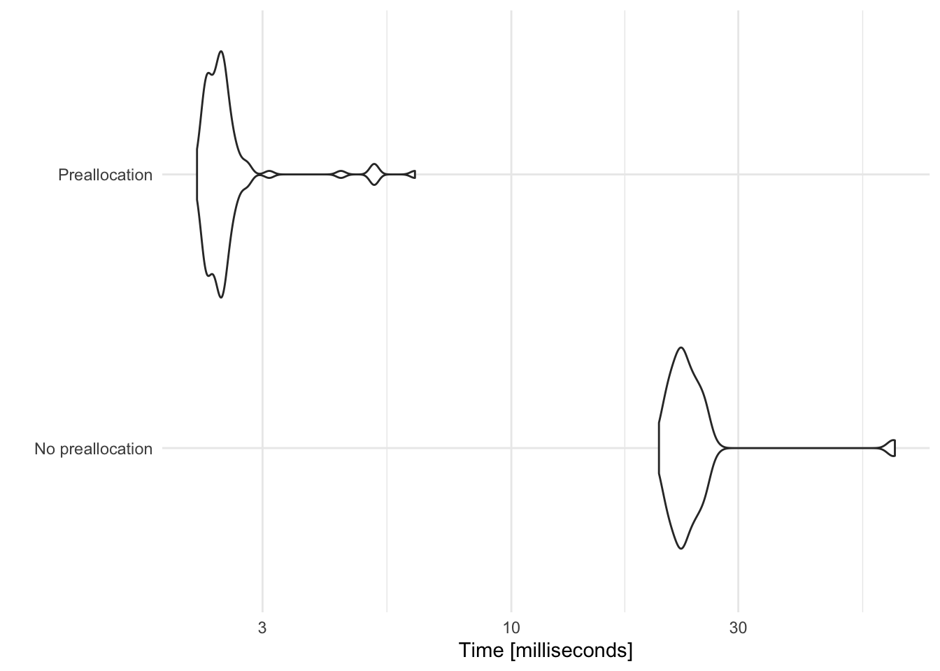
Here, preallocating space for each data frame prior to binding together cuts the computation time by a factor of 10.
Exercise: write a for loop
Mean of columns in car_prices
Write a for loop that calculates the arithmetic mean for every column in modeldata::car_prices.
data("car_prices", package = "modeldata")
car_prices
## # A tibble: 804 × 18
## Price Mileage Cylin…¹ Doors Cruise Sound Leather Buick Cadil…² Chevy Pontiac
## <dbl> <int> <int> <int> <int> <int> <int> <int> <int> <int> <int>
## 1 22661. 20105 6 4 1 0 0 1 0 0 0
## 2 21725. 13457 6 2 1 1 0 0 0 1 0
## 3 29143. 31655 4 2 1 1 1 0 0 0 0
## 4 30732. 22479 4 2 1 0 0 0 0 0 0
## 5 33359. 17590 4 2 1 1 1 0 0 0 0
## 6 30315. 23635 4 2 1 0 0 0 0 0 0
## 7 33382. 17381 4 2 1 1 1 0 0 0 0
## 8 30251. 27558 4 2 1 0 1 0 0 0 0
## 9 30167. 25049 4 2 1 0 0 0 0 0 0
## 10 27060. 17319 4 4 1 0 1 0 0 0 0
## # … with 794 more rows, 7 more variables: Saab <int>, Saturn <int>,
## # convertible <int>, coupe <int>, hatchback <int>, sedan <int>, wagon <int>,
## # and abbreviated variable names ¹Cylinder, ²Cadillac
## # ℹ Use `print(n = ...)` to see more rows, and `colnames()` to see all variable names
Before you write the for loop, identify the three components you need:
- Output
- Sequence
- Body
Click for the solution
- Output - a numeric vector of length 18
- Sequence -
i in seq_along(car_prices) - Body - calculate the
mean()of the $i$th column, store the new value as the $i$th element of the vectoroutput
# preallocate space for the output
output <- vector("numeric", ncol(car_prices))

# initialize the loop along all the columns of car_prices
for (i in seq_along(car_prices)) {
  # calculate the mean value for the i-th column
  output[[i]] <- mean(car_prices[[i]], na.rm = TRUE)
}

output
##  [1] 2.134314e+04 1.983193e+04 5.268657e+00 3.527363e+00 7.524876e-01
##  [6] 6.791045e-01 7.238806e-01 9.950249e-02 9.950249e-02 3.980100e-01
## [11] 1.865672e-01 1.417910e-01 7.462687e-02 6.218905e-02 1.741294e-01
## [16] 7.462687e-02 6.094527e-01 7.960199e-02
Maximum value in each column of car_prices
Write a for loop that calculates the maximum value in each column of car_prices.
Before you write the for loop, identify the three components you need:
- Output
- Sequence
- Body
Click for the solution
- Output - a vector of length 18
- Sequence -
i in seq_along(car_prices) - Body - get the maximum value of the $i$th column of the data frame
car_prices, store the new value as the $i$th element of the listoutput
# preallocate space for the output
output <- vector("numeric", ncol(car_prices))

# initialize the loop along all the columns of car_prices
for (i in seq_along(car_prices)) {
  # calculate the max value for the i-th column
  output[i] <- max(car_prices[[i]])
}

output
##  [1] 70755.47 50387.00     8.00     4.00     1.00     1.00     1.00     1.00
##  [9]     1.00     1.00     1.00     1.00     1.00     1.00     1.00     1.00
## [17]     1.00     1.00
To preserve the name attributes from car_prices, use the names() function to extract the names of each column in car_prices and apply them as the names to the output vector:
# get the names of the columns in car_prices
names(car_prices)
##  [1] "Price"       "Mileage"     "Cylinder"    "Doors"       "Cruise"
##  [6] "Sound"       "Leather"     "Buick"       "Cadillac"    "Chevy"
## [11] "Pontiac"     "Saab"        "Saturn"      "convertible" "coupe"
## [16] "hatchback"   "sedan"       "wagon"
# assign the names of the car_prices columns to output
names(output) <- names(car_prices)
output
##       Price     Mileage    Cylinder       Doors      Cruise       Sound
##    70755.47    50387.00        8.00        4.00        1.00        1.00
##     Leather       Buick    Cadillac       Chevy     Pontiac        Saab
##        1.00        1.00        1.00        1.00        1.00        1.00
##      Saturn convertible       coupe   hatchback       sedan       wagon
##        1.00        1.00        1.00        1.00        1.00        1.00
Map functions
You will frequently need to iterate over vectors or data frames, perform an operation on each element, and save the results somewhere. for loops are not the devil. At first, they may seem more intuitive to use because you are explicitly identifying each component of the process. However the downside is that they focus on a lot of non-essential stuff. You have to track the value on which you are iterating, you need to explicitly create a vector to store the output, you have to assign the output of each iteration to the appropriate element in the output vector, etc.

tidyverse is all about focusing on verbs, not nouns. That is, focus on the operation being performed (e.g. mean(), median(), max()), not all the extra code needed to make the operation work. The purrr library provides a family of functions that mirrors for loops. They:
- Loop over a vector
- Do something to each element
- Save the results

There is one function for each type of output:
map()makes a list.map_lgl()makes a logical vector.map_int()makes an integer vector.map_dbl()makes a double vector.map_chr()makes a character vector.
map_dbl(df, mean)
##          a          b          c          d
## -0.3831574 -0.1181707 -0.3879468 -0.7661931
map_dbl(df, median)
##          a          b          c          d
## -0.5555419 -0.4941011 -0.4656169 -0.6053490
map_dbl(df, sd)
##         a         b         c         d
## 0.9957875 1.0673376 0.6660013 0.8942458
Just like all of our functions in the tidyverse, the first argument is always the data object, and the second argument is the function to be applied. Additional arguments for the function to be applied can be specified like this:
map_dbl(df, mean, na.rm = TRUE)
##          a          b          c          d
## -0.3831574 -0.1181707 -0.3879468 -0.7661931
Or data can be piped:
df %>%
  map_dbl(mean, na.rm = TRUE)
##          a          b          c          d
## -0.3831574 -0.1181707 -0.3879468 -0.7661931
Exercise: rewrite our for loops using a map() function
Mean of columns in car_prices
Write a map() function that calculates the arithmetic mean for every column in car_prices.
car_prices
## # A tibble: 804 × 18
## Price Mileage Cylin…¹ Doors Cruise Sound Leather Buick Cadil…² Chevy Pontiac
## <dbl> <int> <int> <int> <int> <int> <int> <int> <int> <int> <int>
## 1 22661. 20105 6 4 1 0 0 1 0 0 0
## 2 21725. 13457 6 2 1 1 0 0 0 1 0
## 3 29143. 31655 4 2 1 1 1 0 0 0 0
## 4 30732. 22479 4 2 1 0 0 0 0 0 0
## 5 33359. 17590 4 2 1 1 1 0 0 0 0
## 6 30315. 23635 4 2 1 0 0 0 0 0 0
## 7 33382. 17381 4 2 1 1 1 0 0 0 0
## 8 30251. 27558 4 2 1 0 1 0 0 0 0
## 9 30167. 25049 4 2 1 0 0 0 0 0 0
## 10 27060. 17319 4 4 1 0 1 0 0 0 0
## # … with 794 more rows, 7 more variables: Saab <int>, Saturn <int>,
## # convertible <int>, coupe <int>, hatchback <int>, sedan <int>, wagon <int>,
## # and abbreviated variable names ¹Cylinder, ²Cadillac
## # ℹ Use `print(n = ...)` to see more rows, and `colnames()` to see all variable names
Click for the solution
map_dbl(car_prices, mean)
##        Price      Mileage     Cylinder        Doors       Cruise        Sound
## 2.134314e+04 1.983193e+04 5.268657e+00 3.527363e+00 7.524876e-01 6.791045e-01
##      Leather        Buick     Cadillac        Chevy      Pontiac         Saab
## 7.238806e-01 9.950249e-02 9.950249e-02 3.980100e-01 1.865672e-01 1.417910e-01
##       Saturn  convertible        coupe    hatchback        sedan        wagon
## 7.462687e-02 6.218905e-02 1.741294e-01 7.462687e-02 6.094527e-01 7.960199e-02
Maximum value in each column of car_prices
Write a map() function that calculates the maximum value in each column of car_prices.
Click for the solution
map_dbl(car_prices, max)
##       Price     Mileage    Cylinder       Doors      Cruise       Sound
##    70755.47    50387.00        8.00        4.00        1.00        1.00
##     Leather       Buick    Cadillac       Chevy     Pontiac        Saab
##        1.00        1.00        1.00        1.00        1.00        1.00
##      Saturn convertible       coupe   hatchback       sedan       wagon
##        1.00        1.00        1.00        1.00        1.00        1.00
across()
When working with data frames, it’s often useful to perform the same operation on multiple columns. For instance, calculating the average value of each column in car_prices. If we want to calculate the average of a single column, it would be pretty simple to do so just by using tidyverse functions:
car_prices %>%
  summarize(Price = mean(Price))
## # A tibble: 1 × 1
##    Price
##    <dbl>
## 1 21343.
If we want to calculate the mean for all of the columns, we would have to duplicate this code many times over:
car_prices %>%
  summarize(
    Price = mean(Price),
    Mileage = mean(Mileage),
    Cylinder = mean(Cylinder),
    Doors = mean(Doors),
    Cruise = mean(Cruise),
    Sound = mean(Sound),
    Leather = mean(Leather),
    Buick = mean(Buick),
    Cadillac = mean(Cadillac),
    Chevy = mean(Chevy),
    Pontiac = mean(Pontiac),
    Saab = mean(Saab),
    Saturn = mean(Saturn),
    convertible = mean(convertible),
    coupe = mean(coupe),
    hatchback = mean(hatchback),
    sedan = mean(sedan),
    wagon = mean(wagon)
  )
## # A tibble: 1 × 18
## Price Mileage Cylin…¹ Doors Cruise Sound Leather Buick Cadil…² Chevy Pontiac
## <dbl> <dbl> <dbl> <dbl> <dbl> <dbl> <dbl> <dbl> <dbl> <dbl> <dbl>
## 1 21343. 19832. 5.27 3.53 0.752 0.679 0.724 0.0995 0.0995 0.398 0.187
## # … with 7 more variables: Saab <dbl>, Saturn <dbl>, convertible <dbl>,
## # coupe <dbl>, hatchback <dbl>, sedan <dbl>, wagon <dbl>, and abbreviated
## # variable names ¹Cylinder, ²Cadillac
## # ℹ Use `colnames()` to see all variable names
But this process is very repetitive and prone to mistakes - I cannot tell you how many typos I originally had in this code when I first wrote it.
We’ve seen how to use loops and map() functions to solve this task - let’s check out one final method: the across() function.
across() makes it easy to apply the same transformation to multiple columns, allowing you to use select() semantics inside summarize() and mutate(), and other dplyr verbs (or functions).
across() has two primary arguments:
- The first argument,
.cols, selects the columns you want to operate on. It uses tidy selection (likeselect()) so you can pick variables by position, name, and type. - The second argument,
.fns, is a function or list of functions to apply to each column. This can also be apurrrstyle formula (or list of formulas) like~ .x / 2.
Here are a couple of examples of across() in conjunction with its favorite verb, summarize():
Summarize
summarize(), across(), and everything()
To apply a function to each column in a tibble, use across() in conjunction with everything(). everything() is a selection helper that selects all the variables in a data frame. It should be the first argument in across().
car_prices %>%
  summarize(across(.cols = everything(), .fns = mean))
## # A tibble: 1 × 18
## Price Mileage Cylin…¹ Doors Cruise Sound Leather Buick Cadil…² Chevy Pontiac
## <dbl> <dbl> <dbl> <dbl> <dbl> <dbl> <dbl> <dbl> <dbl> <dbl> <dbl>
## 1 21343. 19832. 5.27 3.53 0.752 0.679 0.724 0.0995 0.0995 0.398 0.187
## # … with 7 more variables: Saab <dbl>, Saturn <dbl>, convertible <dbl>,
## # coupe <dbl>, hatchback <dbl>, sedan <dbl>, wagon <dbl>, and abbreviated
## # variable names ¹Cylinder, ²Cadillac
## # ℹ Use `colnames()` to see all variable names
If you want to apply multiple summaries, you store the functions in a list():
car_prices %>%
  summarize(across(everything(), .fns = list(min, max)))
## # A tibble: 1 × 36
##   Price_1 Price_2 Mileage_1 Mileage_2 Cylinder_1 Cylin…¹ Doors_1 Doors_2 Cruis…²
##     <dbl>   <dbl>     <int>     <int>      <int>   <int>   <int>   <int>   <int>
## 1   8639.  70755.       266     50387          4       8       2       4       0
## # … with 27 more variables: Cruise_2 <int>, Sound_1 <int>, Sound_2 <int>,
## #   Leather_1 <int>, Leather_2 <int>, Buick_1 <int>, Buick_2 <int>,
## #   Cadillac_1 <int>, Cadillac_2 <int>, Chevy_1 <int>, Chevy_2 <int>,
## #   Pontiac_1 <int>, Pontiac_2 <int>, Saab_1 <int>, Saab_2 <int>,
## #   Saturn_1 <int>, Saturn_2 <int>, convertible_1 <int>, convertible_2 <int>,
## #   coupe_1 <int>, coupe_2 <int>, hatchback_1 <int>, hatchback_2 <int>,
## #   sedan_1 <int>, sedan_2 <int>, wagon_1 <int>, wagon_2 <int>, and …
## # ℹ Use `colnames()` to see all variable names
To clearly distinguish each summarized variable, we can name them in the list:
car_prices %>%
  summarize(across(everything(), .fns = list(min = min, max = max)))
## # A tibble: 1 × 36
##   Price_min Price_max Mileage_…¹ Milea…² Cylin…³ Cylin…⁴ Doors…⁵ Doors…⁶ Cruis…⁷
##       <dbl>     <dbl>      <int>   <int>   <int>   <int>   <int>   <int>   <int>
## 1     8639.    70755.        266   50387       4       8       2       4       0
## # … with 27 more variables: Cruise_max <int>, Sound_min <int>, Sound_max <int>,
## #   Leather_min <int>, Leather_max <int>, Buick_min <int>, Buick_max <int>,
## #   Cadillac_min <int>, Cadillac_max <int>, Chevy_min <int>, Chevy_max <int>,
## #   Pontiac_min <int>, Pontiac_max <int>, Saab_min <int>, Saab_max <int>,
## #   Saturn_min <int>, Saturn_max <int>, convertible_min <int>,
## #   convertible_max <int>, coupe_min <int>, coupe_max <int>,
## #   hatchback_min <int>, hatchback_max <int>, sedan_min <int>, …
## # ℹ Use `colnames()` to see all variable names
Because across() is usually used in combination with summarise() and mutate(), it does not select grouping variables in order to avoid accidentally modifying them:
car_prices %>%
  group_by(Cylinder) %>%
  summarize(across(everything(), .fns = mean))
## # A tibble: 3 × 18
## Cylinder Price Mileage Doors Cruise Sound Leather Buick Cadil…¹ Chevy Pontiac
## <int> <dbl> <dbl> <dbl> <dbl> <dbl> <dbl> <dbl> <dbl> <dbl> <dbl>
## 1 4 17863. 20108. 3.44 0.599 0.698 0.746 0 0 0.457 0.127
## 2 6 20081. 19564. 3.74 0.868 0.706 0.606 0.258 0.0645 0.387 0.258
## 3 8 38968. 19575. 3.2 1 0.52 1 0 0.6 0.2 0.2
## # … with 7 more variables: Saab <dbl>, Saturn <dbl>, convertible <dbl>,
## # coupe <dbl>, hatchback <dbl>, sedan <dbl>, wagon <dbl>, and abbreviated
## # variable name ¹Cadillac
## # ℹ Use `colnames()` to see all variable names
summarize() and across()
As mentioned earlier, across() allows you to pick variables by position and name:
# pick by name
worldbank %>%
  summarize(across(.cols = life_exp, .fns = mean))
## # A tibble: 1 × 1
##   life_exp
##      <dbl>
## 1     76.6
# by position
worldbank %>%
  summarize(across(.cols = 12, .fns = mean))
## # A tibble: 1 × 1
##   life_exp
##      <dbl>
## 1     76.6
By default, the newly created columns have the shortest names needed to uniquely identify the output.
worldbank %>%
  summarize(across(.cols = life_exp, .fns = list(min, max)))
## # A tibble: 1 × 2
##   life_exp_1 life_exp_2
##        <dbl>      <dbl>
## 1       67.3       82.6
worldbank %>%
  summarize(across(.cols = c(life_exp, pop_growth), .fns = min))
## # A tibble: 1 × 2
##   life_exp pop_growth
##      <dbl>      <dbl>
## 1     67.3      0.479
worldbank %>%
  summarize(across(.cols = -life_exp, .fns = list(min, max)))
## # A tibble: 1 × 26
##   iso3c_1 iso3c_2 date_1 date_2 iso2c_1 iso2c_2 country_1 country_2
##   <chr>   <chr>   <chr>  <chr>  <chr>   <chr>   <chr>     <chr>
## 1 ARG     USA     2005   2017   AR      US      Argentina United States
## # … with 18 more variables: perc_energy_fosfuel_1 <dbl>,
## #   perc_energy_fosfuel_2 <dbl>, rnd_gdpshare_1 <dbl>, rnd_gdpshare_2 <dbl>,
## #   percgni_adj_gross_savings_1 <dbl>, percgni_adj_gross_savings_2 <dbl>,
## #   real_netinc_percap_1 <dbl>, real_netinc_percap_2 <dbl>, gdp_capita_1 <dbl>,
## #   gdp_capita_2 <dbl>, top10perc_incshare_1 <dbl>, top10perc_incshare_2 <dbl>,
## #   employment_ratio_1 <dbl>, employment_ratio_2 <dbl>, pop_growth_1 <dbl>,
## #   pop_growth_2 <dbl>, pop_1 <dbl>, pop_2 <dbl>
summarize(), across(), and where()
To pick variables to summarize based on type, use across() in conjunction with where().
where() is another selection helper that allows you to pick variables based on a predicate function like is.numeric() or is.character(). For example, if you want to apply a numeric summary function only to numeric columns:
worldbank %>%
  group_by(country) %>%
  summarize(across(.cols = where(is.numeric), .fns = mean, na.rm = TRUE))
## # A tibble: 6 × 11
## country perc_…¹ rnd_g…² percg…³ real_…⁴ gdp_c…⁵ top10…⁶ emplo…⁷ life_…⁸
## <chr> <dbl> <dbl> <dbl> <dbl> <dbl> <dbl> <dbl> <dbl>
## 1 Argentina 89.1 0.501 17.5 8560. 10648. 31.6 55.4 75.4
## 2 China 87.6 1.67 48.3 3661. 5397. 30.8 69.8 74.7
## 3 Indonesia 65.3 0.0841 30.5 2041. 2881. 31.2 62.5 69.5
## 4 Norway 58.9 1.60 37.2 70775. 85622. 21.9 67.3 81.3
## 5 United Kingdom 86.3 1.68 13.5 34542. 43416. 26.2 58.7 80.4
## 6 United States 84.2 2.69 17.6 42824. 51285. 30.1 60.2 78.4
## # … with 2 more variables: pop_growth <dbl>, pop <dbl>, and abbreviated
## # variable names ¹perc_energy_fosfuel, ²rnd_gdpshare,
## # ³percgni_adj_gross_savings, ⁴real_netinc_percap, ⁵gdp_capita,
## # ⁶top10perc_incshare, ⁷employment_ratio, ⁸life_exp
## # ℹ Use `colnames()` to see all variable names
(Note that na.rm = TRUE is passed on to mean() in the same way as in purrr::map().)
across() also allows you to create compound selections. For example, you can now transform all numeric columns whose name begins with “perc”:
worldbank %>%
  group_by(country) %>%
  summarize(across(
    .cols = where(is.numeric) & starts_with("perc"),
    .fn = mean, na.rm = TRUE
  ))
## # A tibble: 6 × 3
##   country        perc_energy_fosfuel percgni_adj_gross_savings
##   <chr>                        <dbl>                     <dbl>
## 1 Argentina                     89.1                      17.5
## 2 China                         87.6                      48.3
## 3 Indonesia                     65.3                      30.5
## 4 Norway                        58.9                      37.2
## 5 United Kingdom                86.3                      13.5
## 6 United States                 84.2                      17.6
Mutate
Combinations of mutate() and across() work in a similar way to their summarize equivalents.
car_prices %>%
  mutate(across(.cols = Price:Doors, .fns = log10))
## # A tibble: 804 × 18
## Price Mileage Cylinder Doors Cruise Sound Leather Buick Cadil…¹ Chevy Pontiac
## <dbl> <dbl> <dbl> <dbl> <int> <int> <int> <int> <int> <int> <int>
## 1 4.36 4.30 0.778 0.602 1 0 0 1 0 0 0
## 2 4.34 4.13 0.778 0.301 1 1 0 0 0 1 0
## 3 4.46 4.50 0.602 0.301 1 1 1 0 0 0 0
## 4 4.49 4.35 0.602 0.301 1 0 0 0 0 0 0
## 5 4.52 4.25 0.602 0.301 1 1 1 0 0 0 0
## 6 4.48 4.37 0.602 0.301 1 0 0 0 0 0 0
## 7 4.52 4.24 0.602 0.301 1 1 1 0 0 0 0
## 8 4.48 4.44 0.602 0.301 1 0 1 0 0 0 0
## 9 4.48 4.40 0.602 0.301 1 0 0 0 0 0 0
## 10 4.43 4.24 0.602 0.602 1 0 1 0 0 0 0
## # … with 794 more rows, 7 more variables: Saab <int>, Saturn <int>,
## # convertible <int>, coupe <int>, hatchback <int>, sedan <int>, wagon <int>,
## # and abbreviated variable name ¹Cadillac
## # ℹ Use `print(n = ...)` to see more rows, and `colnames()` to see all variable names
Filter
We cannot directly use across() in filter() because we need an extra step to combine the results. To that end, filter() has two special purpose companion functions:
if_any()keeps the rows where the predicate is true for at least one selected column:worldbank %>% filter(if_any(everything(), ~ !is.na(.x)))## # A tibble: 78 × 14 ## iso3c date iso2c country perc_en…¹ rnd_g…² percg…³ real_…⁴ gdp_c…⁵ top10…⁶ ## <chr> <chr> <chr> <chr> <dbl> <dbl> <dbl> <dbl> <dbl> <dbl> ## 1 ARG 2005 AR Argentina 89.1 0.379 15.5 6198. 5110. 35 ## 2 ARG 2006 AR Argentina 88.7 0.400 22.1 7388. 5919. 33.9 ## 3 ARG 2007 AR Argentina 89.2 0.402 22.8 8182. 7245. 33.8 ## 4 ARG 2008 AR Argentina 90.7 0.421 21.6 8576. 9021. 32.5 ## 5 ARG 2009 AR Argentina 89.6 0.519 18.9 7904. 8225. 31.4 ## 6 ARG 2010 AR Argentina 89.5 0.518 17.9 8803. 10386. 32 ## 7 ARG 2011 AR Argentina 88.9 0.537 17.9 9528. 12849. 31 ## 8 ARG 2012 AR Argentina 89.0 0.609 16.5 9301. 13083. 29.7 ## 9 ARG 2013 AR Argentina 89.0 0.612 15.3 9367. 13080. 29.4 ## 10 ARG 2014 AR Argentina 87.7 0.613 16.1 8903. 12335. 29.9 ## # … with 68 more rows, 4 more variables: employment_ratio <dbl>, ## # life_exp <dbl>, pop_growth <dbl>, pop <dbl>, and abbreviated variable names ## # ¹perc_energy_fosfuel, ²rnd_gdpshare, ³percgni_adj_gross_savings, ## # ⁴real_netinc_percap, ⁵gdp_capita, ⁶top10perc_incshare ## # ℹ Use `print(n = ...)` to see more rows, and `colnames()` to see all variable namesif_all()keeps the rows where the predicate is true for all selected columns:worldbank %>% filter(if_all(everything(), ~ !is.na(.x)))## # A tibble: 42 × 14 ## iso3c date iso2c country perc_en…¹ rnd_g…² percg…³ real_…⁴ gdp_c…⁵ top10…⁶ ## <chr> <chr> <chr> <chr> <dbl> <dbl> <dbl> <dbl> <dbl> <dbl> ## 1 ARG 2005 AR Argentina 89.1 0.379 15.5 6198. 5110. 35 ## 2 ARG 2006 AR Argentina 88.7 0.400 22.1 7388. 5919. 33.9 ## 3 ARG 2007 AR Argentina 89.2 0.402 22.8 8182. 7245. 33.8 ## 4 ARG 2008 AR Argentina 90.7 0.421 21.6 8576. 9021. 32.5 ## 5 ARG 2009 AR Argentina 89.6 0.519 18.9 7904. 8225. 31.4 ## 6 ARG 2010 AR Argentina 89.5 0.518 17.9 8803. 10386. 32 ## 7 ARG 2011 AR Argentina 88.9 0.537 17.9 9528. 12849. 31 ## 8 ARG 2012 AR Argentina 89.0 0.609 16.5 9301. 13083. 29.7 ## 9 ARG 2013 AR Argentina 89.0 0.612 15.3 9367. 13080. 29.4 ## 10 ARG 2014 AR Argentina 87.7 0.613 16.1 8903. 12335. 29.9 ## # … with 32 more rows, 4 more variables: employment_ratio <dbl>, ## # life_exp <dbl>, pop_growth <dbl>, pop <dbl>, and abbreviated variable names ## # ¹perc_energy_fosfuel, ²rnd_gdpshare, ³percgni_adj_gross_savings, ## # ⁴real_netinc_percap, ⁵gdp_capita, ⁶top10perc_incshare ## # ℹ Use `print(n = ...)` to see more rows, and `colnames()` to see all variable names
Exercise: iterate over columns using across()
Rescale numeric variables
Use across() to rescale all numeric variables in rcis::worldbank to range between 0 and 1. You can reuse the function from R for Data Science.
rescale01 <- function(x) {
  rng <- range(x, na.rm = TRUE)
  (x - rng[1]) / (rng[2] - rng[1])
}
Click for the solution
worldbank %>%
  mutate(across(.cols = where(is.numeric), .fns = rescale01))
## # A tibble: 78 × 14
## iso3c date iso2c country perc_en…¹ rnd_g…² percg…³ real_…⁴ gdp_c…⁵ top10…⁶
## <chr> <chr> <chr> <chr> <dbl> <dbl> <dbl> <dbl> <dbl> <dbl>
## 1 ARG 2005 AR Argentina 0.955 0.108 0.0944 0.0938 0.0378 1
## 2 ARG 2006 AR Argentina 0.944 0.116 0.262 0.110 0.0458 0.924
## 3 ARG 2007 AR Argentina 0.960 0.116 0.279 0.121 0.0589 0.917
## 4 ARG 2008 AR Argentina 1 0.124 0.249 0.126 0.0763 0.828
## 5 ARG 2009 AR Argentina 0.971 0.159 0.180 0.117 0.0685 0.752
## 6 ARG 2010 AR Argentina 0.968 0.159 0.156 0.129 0.0897 0.793
## 7 ARG 2011 AR Argentina 0.950 0.166 0.154 0.139 0.114 0.724
## 8 ARG 2012 AR Argentina 0.954 0.192 0.120 0.136 0.116 0.634
## 9 ARG 2013 AR Argentina 0.953 0.193 0.0907 0.137 0.116 0.614
## 10 ARG 2014 AR Argentina 0.918 0.194 0.110 0.130 0.109 0.648
## # … with 68 more rows, 4 more variables: employment_ratio <dbl>,
## # life_exp <dbl>, pop_growth <dbl>, pop <dbl>, and abbreviated variable names
## # ¹perc_energy_fosfuel, ²rnd_gdpshare, ³percgni_adj_gross_savings,
## # ⁴real_netinc_percap, ⁵gdp_capita, ⁶top10perc_incshare
## # ℹ Use `print(n = ...)` to see more rows, and `colnames()` to see all variable names
Acknowledgments
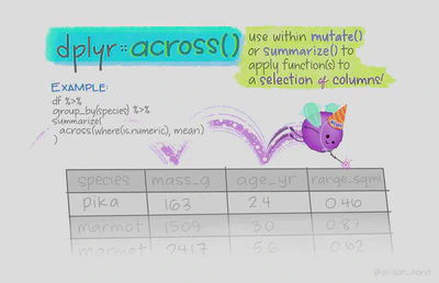
across()based on Column-wise operation vignette- Artwork by @allison_horst
Session Info
sessioninfo::session_info()
## ─ Session info ───────────────────────────────────────────────────────────────
##  setting  value
##  version  R version 4.2.1 (2022-06-23)
##  os       macOS Monterey 12.3
##  system   aarch64, darwin20
##  ui       X11
##  language (EN)
##  collate  en_US.UTF-8
##  ctype    en_US.UTF-8
##  tz       America/New_York
##  date     2022-08-30
##  pandoc   2.18 @ /Applications/RStudio.app/Contents/MacOS/quarto/bin/tools/ (via rmarkdown)
##
## ─ Packages ───────────────────────────────────────────────────────────────────
##  package        * version    date (UTC) lib source
##  assertthat       0.2.1      2019-03-21 [2] CRAN (R 4.2.0)
##  backports        1.4.1      2021-12-13 [2] CRAN (R 4.2.0)
##  blogdown         1.10       2022-05-10 [2] CRAN (R 4.2.0)
##  bookdown         0.27       2022-06-14 [2] CRAN (R 4.2.0)
##  broom            1.0.0      2022-07-01 [2] CRAN (R 4.2.0)
##  bslib            0.4.0      2022-07-16 [2] CRAN (R 4.2.0)
##  cachem           1.0.6      2021-08-19 [2] CRAN (R 4.2.0)
##  cellranger       1.1.0      2016-07-27 [2] CRAN (R 4.2.0)
##  cli              3.3.0      2022-04-25 [2] CRAN (R 4.2.0)
##  codetools        0.2-18     2020-11-04 [2] CRAN (R 4.2.1)
##  colorspace       2.0-3      2022-02-21 [2] CRAN (R 4.2.0)
##  crayon           1.5.1      2022-03-26 [2] CRAN (R 4.2.0)
##  DBI              1.1.3      2022-06-18 [2] CRAN (R 4.2.0)
##  dbplyr           2.2.1      2022-06-27 [2] CRAN (R 4.2.0)
##  digest           0.6.29     2021-12-01 [2] CRAN (R 4.2.0)
##  dplyr          * 1.0.9      2022-04-28 [2] CRAN (R 4.2.0)
##  ellipsis         0.3.2      2021-04-29 [2] CRAN (R 4.2.0)
##  evaluate         0.16       2022-08-09 [1] CRAN (R 4.2.1)
##  fansi            1.0.3      2022-03-24 [2] CRAN (R 4.2.0)
##  fastmap          1.1.0      2021-01-25 [2] CRAN (R 4.2.0)
##  forcats        * 0.5.1      2021-01-27 [2] CRAN (R 4.2.0)
##  fs               1.5.2      2021-12-08 [2] CRAN (R 4.2.0)
##  gargle           1.2.0      2021-07-02 [2] CRAN (R 4.2.0)
##  generics         0.1.3      2022-07-05 [2] CRAN (R 4.2.0)
##  ggplot2        * 3.3.6      2022-05-03 [2] CRAN (R 4.2.0)
##  glue             1.6.2      2022-02-24 [2] CRAN (R 4.2.0)
##  googledrive      2.0.0      2021-07-08 [2] CRAN (R 4.2.0)
##  googlesheets4    1.0.0      2021-07-21 [2] CRAN (R 4.2.0)
##  gtable           0.3.0      2019-03-25 [2] CRAN (R 4.2.0)
##  haven            2.5.0      2022-04-15 [2] CRAN (R 4.2.0)
##  here             1.0.1      2020-12-13 [2] CRAN (R 4.2.0)
##  hms              1.1.1      2021-09-26 [2] CRAN (R 4.2.0)
##  htmltools        0.5.3      2022-07-18 [2] CRAN (R 4.2.0)
##  httr             1.4.3      2022-05-04 [2] CRAN (R 4.2.0)
##  jquerylib        0.1.4      2021-04-26 [2] CRAN (R 4.2.0)
##  jsonlite         1.8.0      2022-02-22 [2] CRAN (R 4.2.0)
##  knitr            1.39       2022-04-26 [2] CRAN (R 4.2.0)
##  lifecycle        1.0.1      2021-09-24 [2] CRAN (R 4.2.0)
##  lubridate        1.8.0      2021-10-07 [2] CRAN (R 4.2.0)
##  magrittr         2.0.3      2022-03-30 [2] CRAN (R 4.2.0)
##  microbenchmark * 1.4.9      2021-11-09 [2] CRAN (R 4.2.0)
##  modeldata      * 1.0.0      2022-07-01 [2] CRAN (R 4.2.0)
##  modelr           0.1.8      2020-05-19 [2] CRAN (R 4.2.0)
##  munsell          0.5.0      2018-06-12 [2] CRAN (R 4.2.0)
##  palmerpenguins * 0.1.0      2020-07-23 [2] CRAN (R 4.2.0)
##  pillar           1.8.0      2022-07-18 [2] CRAN (R 4.2.0)
##  pkgconfig        2.0.3      2019-09-22 [2] CRAN (R 4.2.0)
##  purrr          * 0.3.4      2020-04-17 [2] CRAN (R 4.2.0)
##  R6               2.5.1      2021-08-19 [2] CRAN (R 4.2.0)
##  rcfss          * 0.2.5      2022-08-04 [2] local
##  rcis           * 0.2.5      2022-08-08 [2] local
##  readr          * 2.1.2      2022-01-30 [2] CRAN (R 4.2.0)
##  readxl           1.4.0      2022-03-28 [2] CRAN (R 4.2.0)
##  reprex           2.0.1.9000 2022-08-10 [1] Github (tidyverse/reprex@6d3ad07)
##  rlang            1.0.4      2022-07-12 [2] CRAN (R 4.2.0)
##  rmarkdown        2.14       2022-04-25 [2] CRAN (R 4.2.0)
##  rprojroot        2.0.3      2022-04-02 [2] CRAN (R 4.2.0)
##  rstudioapi       0.13       2020-11-12 [2] CRAN (R 4.2.0)
##  rvest            1.0.2      2021-10-16 [2] CRAN (R 4.2.0)
##  sass             0.4.2      2022-07-16 [2] CRAN (R 4.2.0)
##  scales           1.2.0      2022-04-13 [2] CRAN (R 4.2.0)
##  sessioninfo      1.2.2      2021-12-06 [2] CRAN (R 4.2.0)
##  stringi          1.7.8      2022-07-11 [2] CRAN (R 4.2.0)
##  stringr        * 1.4.0      2019-02-10 [2] CRAN (R 4.2.0)
##  tibble         * 3.1.8      2022-07-22 [2] CRAN (R 4.2.0)
##  tidyr          * 1.2.0      2022-02-01 [2] CRAN (R 4.2.0)
##  tidyselect       1.1.2      2022-02-21 [2] CRAN (R 4.2.0)
##  tidyverse      * 1.3.2      2022-07-18 [2] CRAN (R 4.2.0)
##  tzdb             0.3.0      2022-03-28 [2] CRAN (R 4.2.0)
##  utf8             1.2.2      2021-07-24 [2] CRAN (R 4.2.0)
##  vctrs            0.4.1      2022-04-13 [2] CRAN (R 4.2.0)
##  withr            2.5.0      2022-03-03 [2] CRAN (R 4.2.0)
##  xfun             0.31       2022-05-10 [1] CRAN (R 4.2.0)
##  xml2             1.3.3      2021-11-30 [2] CRAN (R 4.2.0)
##  yaml             2.3.5      2022-02-21 [2] CRAN (R 4.2.0)
##
##  [1] /Users/soltoffbc/Library/R/arm64/4.2/library
##  [2] /Library/Frameworks/R.framework/Versions/4.2-arm64/Resources/library
##
## ──────────────────────────────────────────────────────────────────────────────