Functions in R

library(tidyverse)
library(palmerpenguins)

Run the code below in your console to download this exercise as a set of R scripts.

usethis::use_course("cis-ds/pipes-and-functions-in-r")

Functions are an important tool in the computational social scientist’s toolkit. They enable you to avoid repetition and copy-and-paste and greatly increase the efficiency of your code writing.

They are easy to reuse. If an update to the code is necessary, you revise it in one location and the changes propogate to all over components that implement the function.
They are self-documenting. Give your function a good name and you will easily remember the function and its purpose.
They are easy-ier to debug. There are fewer chances to make mistakes because the code only exists in one location. When copying and pasting, you may forget to copy an important line or fail to update a line in one location.

In fact, you have used functions the entire time you have programmed in R. The only difference is that the functions were written for you. tidyr, dplyr, ggplot2, all of these libraries contain major functions for tidying, transforming, and visualizing data. You have the power to write your own functions. Well, if you don’t already you soon will.

Good rule of thumb - if you have copied and pasted a block of code more than twice, it is time to convert it to a function.

Components of a function

Functions have three key components:

A name. This should be informative and describe what the function does
The arguments, or list of inputs, to the function. They go inside the parentheses in function().
The body. This is the block of code within {} that immediately follows function(...), and is the code that you developed to perform the action described in the name using the arguments you provide.

The `rescale` function

Here is a user-generated function from R for Data Science. Analyze it and identify the three key components.

rescale01 <- function(x) {
  rng <- range(x, na.rm = TRUE)
  (x - rng[1]) / (rng[2] - rng[1])
}

rescale01(c(0, 5, 10))

## [1] 0.0 0.5 1.0

rescale01(c(-10, 0, 10))

## [1] 0.0 0.5 1.0

rescale01(c(1, 2, 3, NA, 5))

## [1] 0.00 0.25 0.50   NA 1.00

Click for the solution

Name - rescale01
- This is a function that will rescale a variable from 0 to 1
Arguments
- This function takes one argument x - the variable to be transformed
- We could call the argument whatever we like, but x is a conventional name
- Multiple inputs would be x, y, z, etc., or take on informative names such as data, formula, na.rm, etc.
- You should use what makes sense
Body
- This takes two lines of code
  1. Calculate the range of the variable (its minimum and maximum values) and ignore missing values. Save this as an object called rng.
  2. For each value in the variable, subtract the minimum value in the variable and divide by the difference between the maximum and minimum value. Use arthimetic notation to make sure order of operations is followed.
- By default, whatever is the last thing generated by the function is returned as the output

This function can easily be reused for any numeric variable. Rather than writing out the contents of the function every time, we just use the function itself.

Pythagorean theorem function

Analyze the following function.

Identify the name, arguments, and body
What does it do?
If a = 3 and b = 4, what should we expect the output to be?

pythagorean <- function(a, b) {
  hypotenuse <- sqrt(a^2 + b^2)
  return(hypotenuse)
}

Click for the solution

Name - pythagorean
- Calculates the length of the hypotenuse of a right triangle.
Arguments
- These are the inputs of the function. They go inside function
- This function takes two arguments
  - a - length of one side of a right triangle
  - b - length of another side of a right triangle
Body
- Block of code within {} that immediately follows function(...)
- Here, I wrote two lines of code
  - The first line creates a new object hypotenuse which is the square root of the sum of squares of the two sides of the right triangle (also called the hypotenuse)
  - I then explicitly return hypotenuse as the output of the function. I could also have written the function as:

pythagorean <- function(a, b) {
  hypotenuse <- sqrt(a^2 + b^2)
}

or even:

pythagorean <- function(a, b) {
  sqrt(a^2 + b^2)
}

But I wanted to explicitly identify each step of the code for others to review. Early on in your function writing career, you will want to be more explicit so future you can interpret your own code. As you practice and become more comfortable writing functions, you can be more relaxed in your coding style and documentation.

How to use a function

When using functions, by default the returned object is merely printed to the screen.

pythagorean(a = 3, b = 4)

## [1] 5

If you want it saved, you need to assign it to an object.

(tri_c <- pythagorean(a = 3, b = 4))

## [1] 5

Objects created inside functions

pythagorean(a = 3, b = 4)

## [1] 5

hypotenuse

## Error in eval(expr, envir, enclos): object 'hypotenuse' not found

Why does this generate an error? Why can we not see the results of hypotenuse? After all, it was generated by pythagorean, right?

Objects created inside a function exist within their own environment. Typically you are working in the global environment. You can see all objects that exist in that environment in the top-right panel.

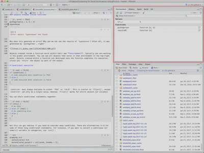
Objects created within a function are destroyed once the function completes its execution, unless you return the object as part of the output. This is why you do not see hypotenuse listed in the environment - it has already been destroyed.

Exercise: calculate the sum of squares of two variables

Write a function that calculates the sum of the squared value of two numbers. For instance, it should generate the following output:

my_function(3, 4)

## [1] 25

Click for the solution

sum_of_squares <- function(x, y) {
  return(x^2 + y^2)
}

sum_of_squares(3, 4)

## [1] 25

Name - sum_of_squares
- Calculates the sum of the squared value of two variables
Arguments
- x - one number
- y - a second number
Body
- The first line squares x and y independently and then adds the results together

Cool fact - this function also works with vectors of numbers

x <- c(2, 4, 6)
y <- c(1, 3, 5)
sum_of_squares(x, y)

## [1]  5 25 61

Conditional execution

Sometimes you only want to execute code if a condition is met. To do that, use an if-else statement.

if (condition) {
  # code executed when condition is TRUE
} else {
  # code executed when condition is FALSE
}

condition must always evaluate to either TRUE or FALSE.¹ This is similar to filter(), except condition can only be a single value (i.e. a vector of length 1), whereas filter() works for entire vectors (or columns).

You can chain conditional statements together:

if (this) {
  # do that
} else if (that) {
  # do something else
} else {
  # do something completely different
}

But this can get tedious if you need to consider many conditions. There are alternatives in R for some of these long conditional statements. For instance, if you want to convert a continuous (or numeric) variable to categories, use cut():

penguins %>%
  select(body_mass_g) %>%
  mutate(
    body_mass_g_autobin = cut(body_mass_g, breaks = 5),
    body_mass_g_manbin = cut(body_mass_g,
      breaks = c(2700, 3600, 4500, 5400, 6300),
      labels = c("Small", "Medium", "Large", "Huge")
    )
  )

## # A tibble: 344 × 3
##    body_mass_g body_mass_g_autobin body_mass_g_manbin
##          <int> <fct>               <fct>             
##  1        3750 (3.42e+03,4.14e+03] Medium            
##  2        3800 (3.42e+03,4.14e+03] Medium            
##  3        3250 (2.7e+03,3.42e+03]  Small             
##  4          NA <NA>                <NA>              
##  5        3450 (3.42e+03,4.14e+03] Small             
##  6        3650 (3.42e+03,4.14e+03] Medium            
##  7        3625 (3.42e+03,4.14e+03] Medium            
##  8        4675 (4.14e+03,4.86e+03] Large             
##  9        3475 (3.42e+03,4.14e+03] Small             
## 10        4250 (4.14e+03,4.86e+03] Medium            
## # … with 334 more rows

`if` versus `if_else()`

Because if-else conditional statements like the ones outlined above must always resolve to a single TRUE or FALSE, they cannot be used for vector operations. Vector operations are where you make multiple comparisons simultaneously for each value stored inside a vector. Consider the gun_deaths data and imagine you wanted to create a new column identifying whether or not an individual had at least a high school education.

library(rcis)

## 
## Attaching package: 'rcis'

## The following objects are masked from 'package:rcfss':
## 
##     add_ci, cfss_notes, cfss_slides, err.rate.rf, err.rate.tree,
##     logit2prob, mse, mse_vec, plot_ci, prob2logodds, prob2odds,
##     xaringan, xaringan_wide

data("gun_deaths")

(educ <- select(gun_deaths, education))

## # A tibble: 100,798 × 1
##    education   
##    <fct>       
##  1 BA+         
##  2 Some college
##  3 BA+         
##  4 BA+         
##  5 HS/GED      
##  6 Less than HS
##  7 HS/GED      
##  8 HS/GED      
##  9 Some college
## 10 <NA>        
## # … with 100,788 more rows

This sounds like a classic if-else operation. For each individual, if education equals “Less than HS”, then the value in the new column should be “Less than HS”. Otherwise, it should be “HS+”. But what happens if we try to implement this using an if-else operation like above?

(educ_if <- educ %>%
  mutate(hsPlus = if (education == "Less than HS") {
    "Less than HS"
  } else {
    "HS+"
  }))

## Error in `mutate()`:
## ! Problem while computing `hsPlus = if (...) NULL`.
## Caused by error in `if (education == "Less than HS") ...`:
## ! the condition has length > 1

This did not work correctly. if() can only handle a single TRUE/FALSE value; as of R version 4.2.0, it generates an error if the argument contains more than a single value.

Because we in fact want to make this if-else comparison 100798 times, we should instead use if_else(). This vectorizes the if-else comparison and makes a separate comparison for each row of the data frame. This allows us to correctly generate this new column.²

educ_ifelse <- educ %>%
  mutate(hsPlus = if_else(
    condition = education == "Less than HS",
    true = "Less than HS",
    false = "HS+"
  ))
educ_ifelse

## # A tibble: 100,798 × 2
##    education    hsPlus      
##    <fct>        <chr>       
##  1 BA+          HS+         
##  2 Some college HS+         
##  3 BA+          HS+         
##  4 BA+          HS+         
##  5 HS/GED       HS+         
##  6 Less than HS Less than HS
##  7 HS/GED       HS+         
##  8 HS/GED       HS+         
##  9 Some college HS+         
## 10 <NA>         <NA>        
## # … with 100,788 more rows
## # ℹ Use `print(n = ...)` to see more rows

count(educ_ifelse, hsPlus)

## # A tibble: 3 × 2
##   hsPlus           n
##   <chr>        <int>
## 1 HS+          77553
## 2 Less than HS 21823
## 3 <NA>          1422

Exercise: write a `fizzbuzz` function

Fizz buzz is a children’s game that teaches about division. Players take turns counting incrementally, replacing any number divisible by three with the word “fizz” and any number divisible by five with the word “buzz”.

Likewise, a fizzbuzz function takes a single number as input. If the number is divisible by three, it returns “fizz”. If it’s divisible by five it returns “buzz”. If it’s divisible by three and five, it returns “fizzbuzz”. Otherwise, it returns the number.

The output of your function should look like this:

my_function(3)

## [1] "fizz"

my_function(5)

## [1] "buzz"

my_function(15)

## [1] "fizzbuzz"

my_function(4)

## [1] 4

A helpful hint about modular division

%% is modular division. It returns the remainder left over after the division, rather than a floating point number.

5 / 3

## [1] 1.666667

5 %% 3

## [1] 2

Click for the solution

fizzbuzz <- function(x) {
  if (x %% 3 == 0 && x %% 5 == 0) {
    return("fizzbuzz")
  } else if (x %% 3 == 0) {
    return("fizz")
  } else if (x %% 5 == 0) {
    return("buzz")
  } else {
    return(x)
  }
}

fizzbuzz(3)

## [1] "fizz"

fizzbuzz(5)

## [1] "buzz"

fizzbuzz(15)

## [1] "fizzbuzz"

fizzbuzz(4)

## [1] 4

Name - fizzbuzz
- Plays a single round of the Fizz Buzz game
Arguments
- x - a number
Body
- Uses modular division and a series of if-else statements to check if x is evenly divisible with 3 and/or 5.
- The first comparison to make checks if x is a “fizzbuzz” (evenly divisible by 3 and 5). This should be the first comparison because it needs to return “fizzbuzz”. If we had this at the end of the comparison chain, the function would prematurely return on “fizz” or “buzz”.
  - If TRUE, then print “fizzbuzz”
- If the first condition is not met, check to see if x is a “fizz” (divisible by 3).
  - If TRUE, then print “fizz”
- If the first two conditions are not met, check to see if x is a “buzz” (divisible by 5).
  - If TRUE, then print “buzz”
- If the first three conditions are all FALSE, then print the original number x.

Session Info

sessioninfo::session_info()

## ─ Session info ───────────────────────────────────────────────────────────────
##  setting  value
##  version  R version 4.2.1 (2022-06-23)
##  os       macOS Monterey 12.3
##  system   aarch64, darwin20
##  ui       X11
##  language (EN)
##  collate  en_US.UTF-8
##  ctype    en_US.UTF-8
##  tz       America/New_York
##  date     2022-09-14
##  pandoc   2.18 @ /Applications/RStudio.app/Contents/MacOS/quarto/bin/tools/ (via rmarkdown)
## 
## ─ Packages ───────────────────────────────────────────────────────────────────
##  package        * version    date (UTC) lib source
##  assertthat       0.2.1      2019-03-21 [2] CRAN (R 4.2.0)
##  backports        1.4.1      2021-12-13 [2] CRAN (R 4.2.0)
##  blogdown         1.10       2022-05-10 [2] CRAN (R 4.2.0)
##  bookdown         0.27       2022-06-14 [2] CRAN (R 4.2.0)
##  broom            1.0.0      2022-07-01 [2] CRAN (R 4.2.0)
##  bslib            0.4.0      2022-07-16 [2] CRAN (R 4.2.0)
##  cachem           1.0.6      2021-08-19 [2] CRAN (R 4.2.0)
##  cellranger       1.1.0      2016-07-27 [2] CRAN (R 4.2.0)
##  cli              3.3.0      2022-04-25 [2] CRAN (R 4.2.0)
##  codetools        0.2-18     2020-11-04 [2] CRAN (R 4.2.1)
##  colorspace       2.0-3      2022-02-21 [2] CRAN (R 4.2.0)
##  crayon           1.5.1      2022-03-26 [2] CRAN (R 4.2.0)
##  DBI              1.1.3      2022-06-18 [2] CRAN (R 4.2.0)
##  dbplyr           2.2.1      2022-06-27 [2] CRAN (R 4.2.0)
##  digest           0.6.29     2021-12-01 [2] CRAN (R 4.2.0)
##  dplyr          * 1.0.9      2022-04-28 [2] CRAN (R 4.2.0)
##  ellipsis         0.3.2      2021-04-29 [2] CRAN (R 4.2.0)
##  evaluate         0.16       2022-08-09 [1] CRAN (R 4.2.1)
##  fansi            1.0.3      2022-03-24 [2] CRAN (R 4.2.0)
##  fastmap          1.1.0      2021-01-25 [2] CRAN (R 4.2.0)
##  forcats        * 0.5.1      2021-01-27 [2] CRAN (R 4.2.0)
##  fs               1.5.2      2021-12-08 [2] CRAN (R 4.2.0)
##  gargle           1.2.0      2021-07-02 [2] CRAN (R 4.2.0)
##  generics         0.1.3      2022-07-05 [2] CRAN (R 4.2.0)
##  ggplot2        * 3.3.6      2022-05-03 [2] CRAN (R 4.2.0)
##  glue             1.6.2      2022-02-24 [2] CRAN (R 4.2.0)
##  googledrive      2.0.0      2021-07-08 [2] CRAN (R 4.2.0)
##  googlesheets4    1.0.0      2021-07-21 [2] CRAN (R 4.2.0)
##  gtable           0.3.0      2019-03-25 [2] CRAN (R 4.2.0)
##  haven            2.5.0      2022-04-15 [2] CRAN (R 4.2.0)
##  here             1.0.1      2020-12-13 [2] CRAN (R 4.2.0)
##  hms              1.1.1      2021-09-26 [2] CRAN (R 4.2.0)
##  htmltools        0.5.3      2022-07-18 [2] CRAN (R 4.2.0)
##  httr             1.4.3      2022-05-04 [2] CRAN (R 4.2.0)
##  jquerylib        0.1.4      2021-04-26 [2] CRAN (R 4.2.0)
##  jsonlite         1.8.0      2022-02-22 [2] CRAN (R 4.2.0)
##  knitr            1.39       2022-04-26 [2] CRAN (R 4.2.0)
##  lifecycle        1.0.1      2021-09-24 [2] CRAN (R 4.2.0)
##  lubridate        1.8.0      2021-10-07 [2] CRAN (R 4.2.0)
##  magrittr         2.0.3      2022-03-30 [2] CRAN (R 4.2.0)
##  modelr           0.1.8      2020-05-19 [2] CRAN (R 4.2.0)
##  munsell          0.5.0      2018-06-12 [2] CRAN (R 4.2.0)
##  palmerpenguins * 0.1.0      2020-07-23 [2] CRAN (R 4.2.0)
##  pillar           1.8.0      2022-07-18 [2] CRAN (R 4.2.0)
##  pkgconfig        2.0.3      2019-09-22 [2] CRAN (R 4.2.0)
##  purrr          * 0.3.4      2020-04-17 [2] CRAN (R 4.2.0)
##  R6               2.5.1      2021-08-19 [2] CRAN (R 4.2.0)
##  rcfss          * 0.2.5      2022-08-04 [2] local
##  rcis           * 0.2.5      2022-08-08 [2] local
##  readr          * 2.1.2      2022-01-30 [2] CRAN (R 4.2.0)
##  readxl           1.4.0      2022-03-28 [2] CRAN (R 4.2.0)
##  reprex           2.0.1.9000 2022-08-10 [1] Github (tidyverse/reprex@6d3ad07)
##  rlang            1.0.4      2022-07-12 [2] CRAN (R 4.2.0)
##  rmarkdown        2.14       2022-04-25 [2] CRAN (R 4.2.0)
##  rprojroot        2.0.3      2022-04-02 [2] CRAN (R 4.2.0)
##  rstudioapi       0.13       2020-11-12 [2] CRAN (R 4.2.0)
##  rvest            1.0.2      2021-10-16 [2] CRAN (R 4.2.0)
##  sass             0.4.2      2022-07-16 [2] CRAN (R 4.2.0)
##  scales           1.2.0      2022-04-13 [2] CRAN (R 4.2.0)
##  sessioninfo      1.2.2      2021-12-06 [2] CRAN (R 4.2.0)
##  stringi          1.7.8      2022-07-11 [2] CRAN (R 4.2.0)
##  stringr        * 1.4.0      2019-02-10 [2] CRAN (R 4.2.0)
##  tibble         * 3.1.8      2022-07-22 [2] CRAN (R 4.2.0)
##  tidyr          * 1.2.0      2022-02-01 [2] CRAN (R 4.2.0)
##  tidyselect       1.1.2      2022-02-21 [2] CRAN (R 4.2.0)
##  tidyverse      * 1.3.2      2022-07-18 [2] CRAN (R 4.2.0)
##  tzdb             0.3.0      2022-03-28 [2] CRAN (R 4.2.0)
##  utf8             1.2.2      2021-07-24 [2] CRAN (R 4.2.0)
##  vctrs            0.4.1      2022-04-13 [2] CRAN (R 4.2.0)
##  withr            2.5.0      2022-03-03 [2] CRAN (R 4.2.0)
##  xfun             0.31       2022-05-10 [1] CRAN (R 4.2.0)
##  xml2             1.3.3      2021-11-30 [2] CRAN (R 4.2.0)
##  yaml             2.3.5      2022-02-21 [2] CRAN (R 4.2.0)
## 
##  [1] /Users/soltoffbc/Library/R/arm64/4.2/library
##  [2] /Library/Frameworks/R.framework/Versions/4.2-arm64/Resources/library
## 
## ──────────────────────────────────────────────────────────────────────────────

These are Boolean logical values - we used them to make comparisons and will talk more next class about logical vectors. ↩︎
Notice that is also preserves missing values in the new column. Remember, any operation performed on a missing value will itself become a missing value. ↩︎

Last updated on Mar 1, 2019

Functions in R

Components of a function

The rescale function

Pythagorean theorem function

How to use a function

Objects created inside functions

Exercise: calculate the sum of squares of two variables

Conditional execution

if versus if_else()

Exercise: write a fizzbuzz function

A helpful hint about modular division

Session Info

The `rescale` function

`if` versus `if_else()`

Exercise: write a `fizzbuzz` function