Working with statistical models
library(tidyverse)
library(tidymodels)
library(rcis)

set.seed(123)

theme_set(theme_minimal())
Run the code below in your console to download this exercise as a set of R scripts.
usethis::use_course("cis-ds/statistical-learning")
Exercise: linear regression with scorecard
Recall the scorecard data set which contains information on U.S. institutions of higher learning.
scorecard
## # A tibble: 1,732 × 14
## unitid name state type admrate satavg cost netcost avgfa…¹ pctpell compr…²
## <dbl> <chr> <chr> <fct> <dbl> <dbl> <dbl> <dbl> <dbl> <dbl> <dbl>
## 1 100654 Alab… AL Publ… 0.918 939 23053 14990 69381 0.702 0.297
## 2 100663 Univ… AL Publ… 0.737 1234 24495 16953 99441 0.351 0.634
## 3 100706 Univ… AL Publ… 0.826 1319 23917 15860 87192 0.254 0.577
## 4 100724 Alab… AL Publ… 0.969 946 21866 13650 64989 0.763 0.328
## 5 100751 The … AL Publ… 0.827 1261 29872 22597 92619 0.177 0.711
## 6 100830 Aubu… AL Publ… 0.904 1082 19849 13987 71343 0.464 0.340
## 7 100858 Aubu… AL Publ… 0.807 1300 31590 24104 96642 0.146 0.791
## 8 100937 Birm… AL Priv… 0.538 1230 32095 22107 56646 0.236 0.691
## 9 101189 Faul… AL Priv… 0.783 1066 34317 20715 54009 0.488 0.329
## 10 101365 Herz… AL Priv… 0.783 NA 30119 26680 54684 0.706 0.28
## # … with 1,722 more rows, 3 more variables: firstgen <dbl>, debt <dbl>,
## # locale <fct>, and abbreviated variable names ¹avgfacsal, ²comprate
## # ℹ Use `print(n = ...)` to see more rows, and `colnames()` to see all variable names
Answer the following questions using the statistical modeling tools you have learned.
What is the relationship between admission rate and cost? Report this relationship using a scatterplot and a linear best-fit line.
Click for the solution
ggplot(scorecard, aes(admrate, cost)) +
  geom_point() +
  geom_smooth(method = "lm")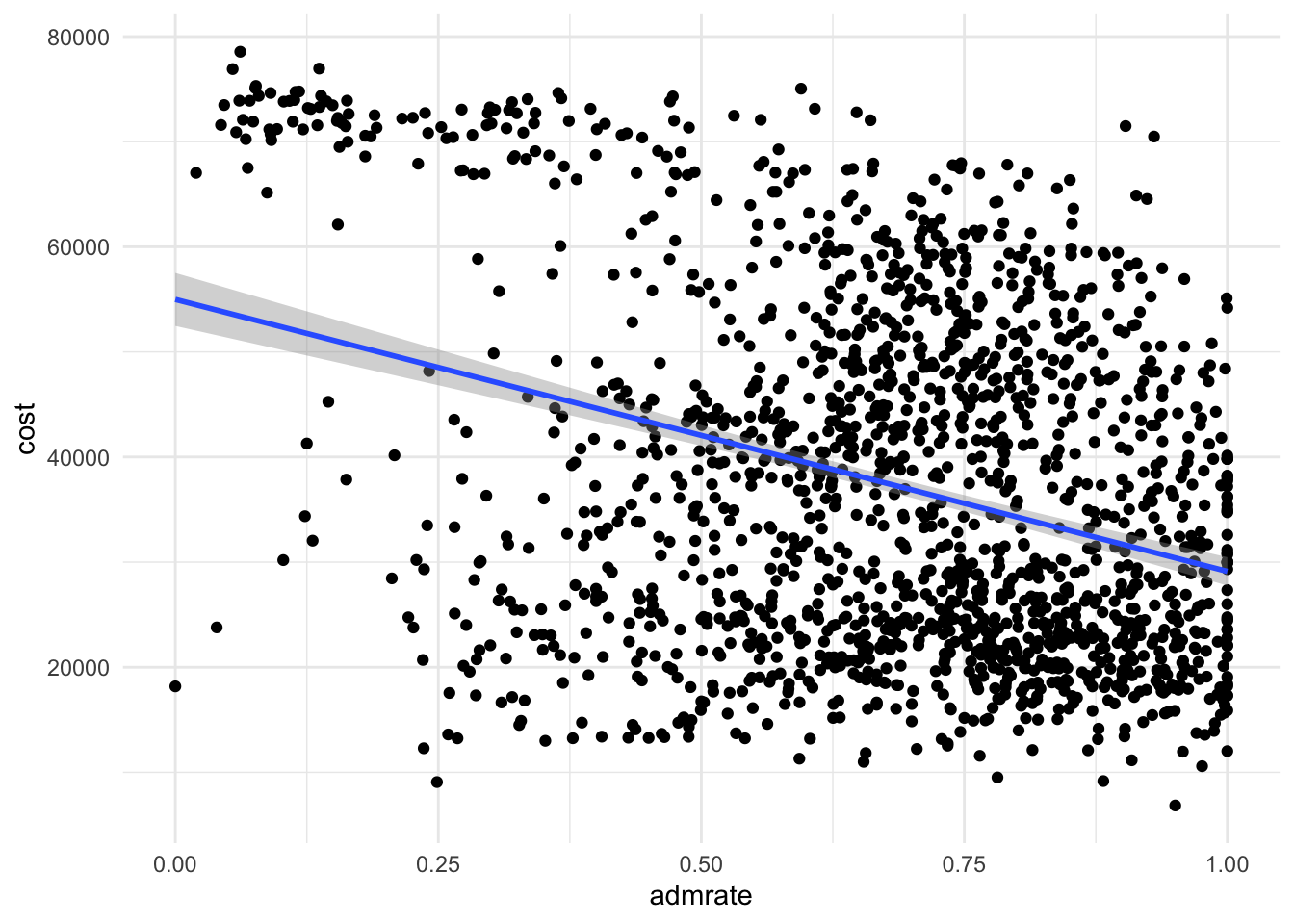
Estimate a linear regression of the relationship between admission rate and cost, and report your results in a tidy table.
Click for the solution
scorecard_fit <- linear_reg() %>%
  set_engine("lm") %>%
  fit(cost ~ admrate, data = scorecard)
tidy(scorecard_fit)
## # A tibble: 2 × 5 ## term estimate std.error statistic p.value ## <chr> <dbl> <dbl> <dbl> <dbl> ## 1 (Intercept) 54992. 1286. 42.8 7.30e-271 ## 2 admrate -25872. 1801. -14.4 3.15e- 44Estimate a linear regression of the relationship between admission rate and cost, while also accounting for type of college and percent of Pell Grant recipients, and report your results in a tidy table.
Click for the solution
scorecard_fit <- linear_reg() %>%
  set_engine("lm") %>%
  fit(cost ~ admrate + type + pctpell, data = scorecard)
tidy(scorecard_fit)
## # A tibble: 5 × 5 ## term estimate std.error statistic p.value ## <chr> <dbl> <dbl> <dbl> <dbl> ## 1 (Intercept) 49319. 1057. 46.6 5.20e-305 ## 2 admrate -13792. 1190. -11.6 6.02e- 30 ## 3 typePrivate, nonprofit 20854. 540. 38.6 1.29e-233 ## 4 typePrivate, for-profit 17390. 1265. 13.7 7.91e- 41 ## 5 pctpell -44530. 1545. -28.8 1.30e-148
Exercise: logistic regression with mental_health
Why do some people vote in elections while others do not? Typical explanations focus on a resource model of participation – individuals with greater resources, such as time, money, and civic skills, are more likely to participate in politics. An emerging theory assesses an individual’s mental health and its effect on political participation.1 Depression increases individuals’ feelings of hopelessness and political efficacy, so depressed individuals will have less desire to participate in politics. More importantly to our resource model of participation, individuals with depression suffer physical ailments such as a lack of energy, headaches, and muscle soreness which drain an individual’s energy and requires time and money to receive treatment. For these reasons, we should expect that individuals with depression are less likely to participate in election than those without symptoms of depression.
Use the mental_health data set in library(rcis) and logistic regression to predict whether or not an individual voted in the 1996 presidential election.
mental_health
## # A tibble: 1,317 × 5
##    vote96   age  educ female mhealth
##     <dbl> <dbl> <dbl>  <dbl>   <dbl>
##  1      1    60    12      0       0
##  2      1    36    12      0       1
##  3      0    21    13      0       7
##  4      0    29    13      0       6
##  5      1    39    18      1       2
##  6      1    41    15      1       1
##  7      1    48    20      0       2
##  8      0    20    12      1       9
##  9      0    27    11      1       9
## 10      0    34     7      1       2
## # … with 1,307 more rows
## # ℹ Use `print(n = ...)` to see more rows
Estimate a logistic regression model of voter turnout with
mhealthas the predictor. Estimate predicted probabilities and a 95% confidence interval, and plot the logistic regression predictions usingggplot.Click for the solution
# convert vote96 to a factor column
mental_health <- rcis::mental_health %>%
  mutate(vote96 = factor(vote96, labels = c("Not voted", "Voted")))
# estimate model mh_mod <- logistic_reg() %>% set_engine("glm") %>% fit(vote96 ~ mhealth, data = mental_health) # generate predicted probabilities + confidence intervals new_points <- tibble( mhealth = seq( from = min(mental_health$mhealth), to = max(mental_health$mhealth) ) ) bind_cols( new_points, # predicted probabilities predict(mh_mod, new_data = new_points, type = "prob"), # confidence intervals predict(mh_mod, new_data = new_points, type = "conf_int") ) %>% # graph the predictions ggplot(mapping = aes(x = mhealth, y = .pred_Voted)) + geom_pointrange(mapping = aes(ymin = .pred_lower_Voted, ymax = .pred_upper_Voted)) + labs( title = "Relationship Between Mental Health and Voter Turnout", x = "Mental health status", y = "Predicted Probability of Voting" )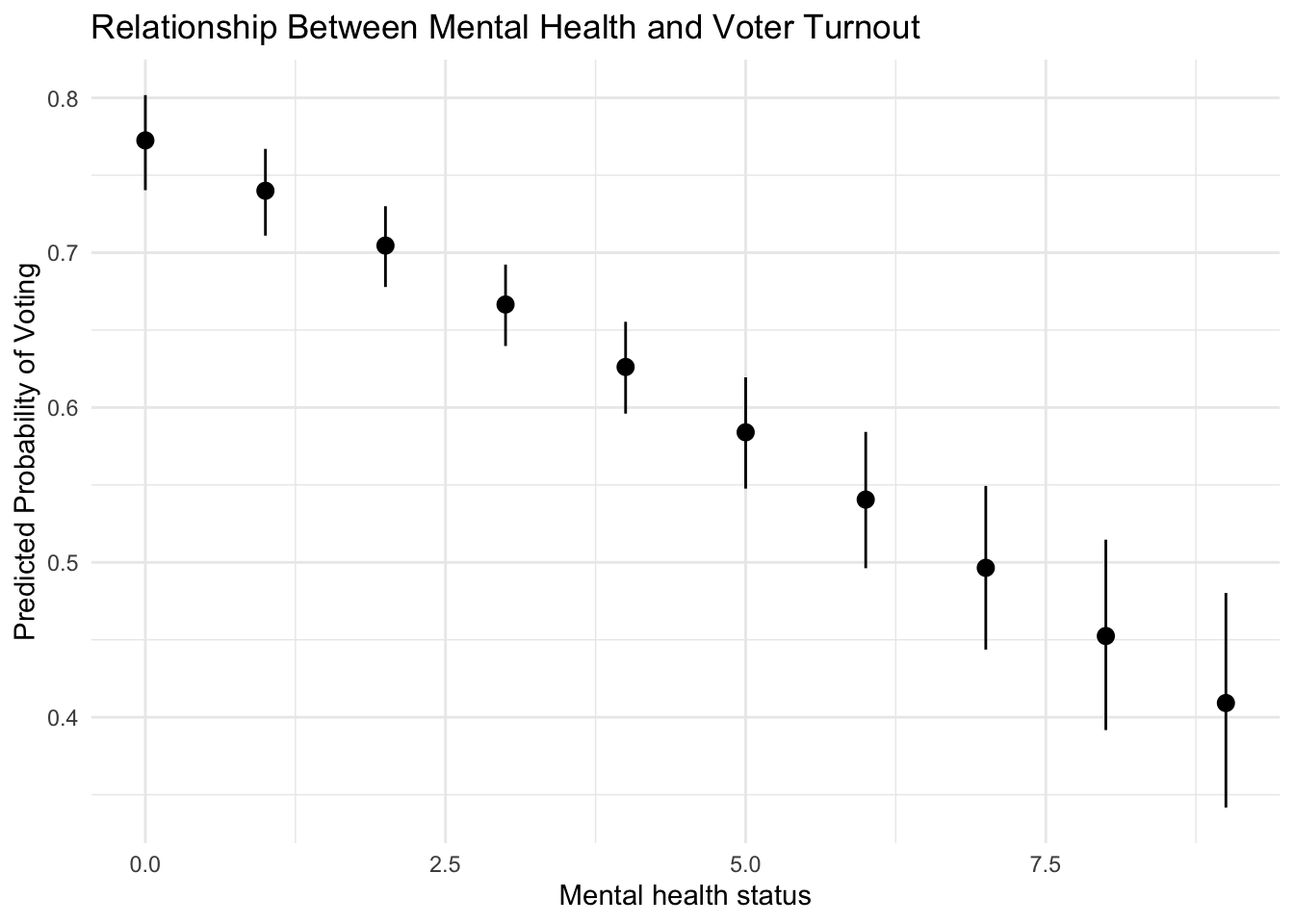
Estimate a second logistic regression model of voter turnout using using age and gender (i.e. the
femalecolumn). Extract predicted probabilities and confidence intervals for all possible values of age, and visualize usingggplot().Click for the solution
# recode female
mental_health <- rcis::mental_health %>%
  mutate(
    vote96 = factor(vote96, labels = c("Not voted", "Voted")),
    female = factor(female, labels = c("Male", "Female"))
  )

# estimate model
mh_int_mod <- logistic_reg() %>%
  set_engine("glm") %>%
  fit(vote96 ~ age * female, data = mental_health)

# generate predicted probabilities + confidence intervals
new_points <- expand.grid(
  age = seq(
    from = min(mental_health$age),
    to = max(mental_health$age)
  ),
  female = unique(mental_health$female)
)

bind_cols(
  new_points,
  # predicted probabilities
  predict(mh_int_mod, new_data = new_points, type = "prob"),
  # confidence intervals
  predict(mh_int_mod, new_data = new_points, type = "conf_int")
) %>%
  # graph the predictions
  ggplot(mapping = aes(x = age, y = .pred_Voted, color = female)) +
  # predicted probability
  geom_line(linetype = 2) +
  # confidence interval
  geom_ribbon(mapping = aes(
    ymin = .pred_lower_Voted, ymax = .pred_upper_Voted,
    fill = female
  ), alpha = .2) +
  scale_color_viridis_d(
    end = 0.7, aesthetics = c("color", "fill"),
    name = NULL
  ) +
  labs(
    title = "Relationship Between Age and Voter Turnout",
    x = "Age",
    y = "Predicted Probability of Voting"
  )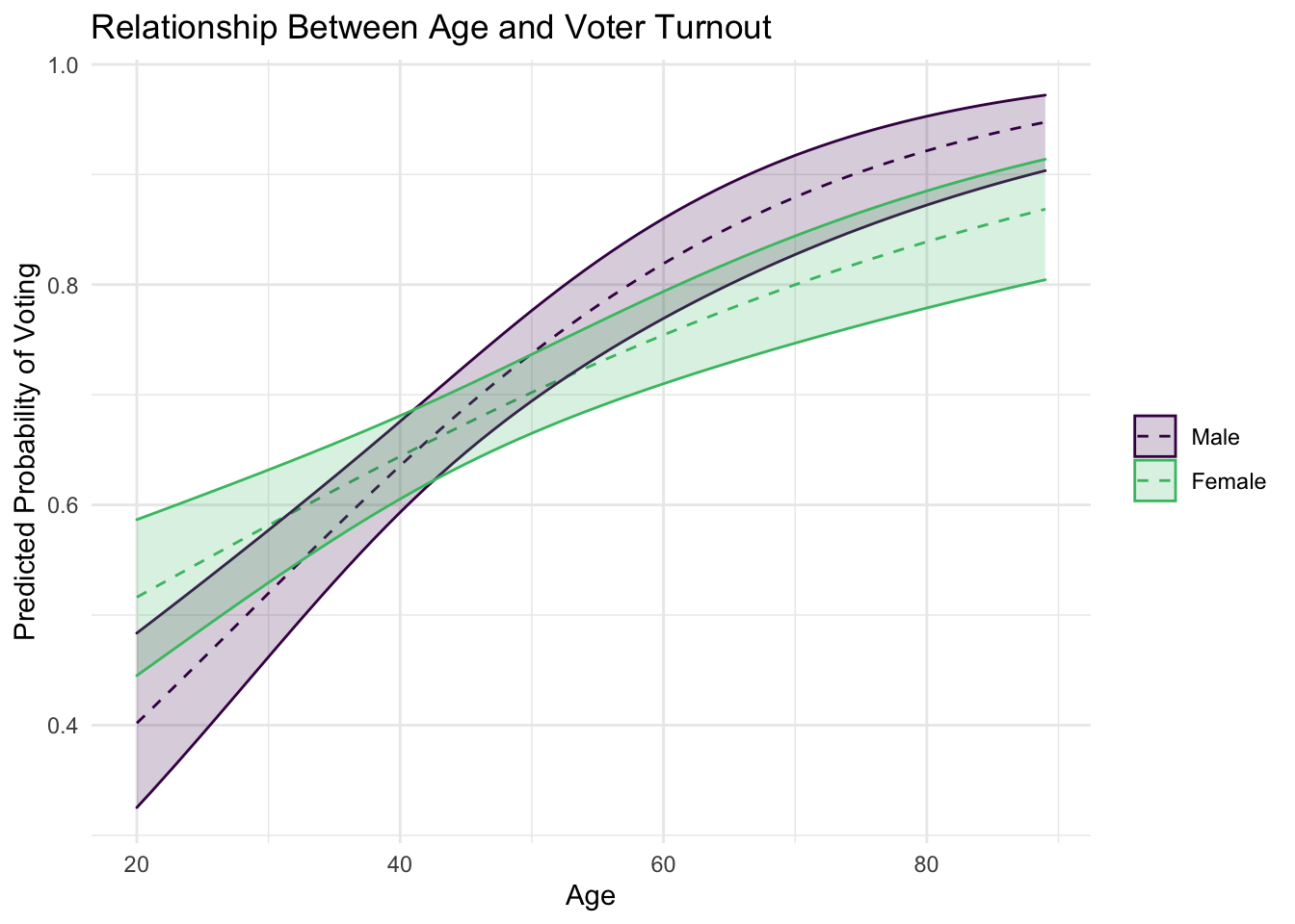
Session Info
sessioninfo::session_info()
## ─ Session info ───────────────────────────────────────────────────────────────
##  setting  value
##  version  R version 4.2.1 (2022-06-23)
##  os       macOS Monterey 12.3
##  system   aarch64, darwin20
##  ui       X11
##  language (EN)
##  collate  en_US.UTF-8
##  ctype    en_US.UTF-8
##  tz       America/New_York
##  date     2022-08-22
##  pandoc   2.18 @ /Applications/RStudio.app/Contents/MacOS/quarto/bin/tools/ (via rmarkdown)
##
## ─ Packages ───────────────────────────────────────────────────────────────────
##  package       * version    date (UTC) lib source
##  assertthat      0.2.1      2019-03-21 [2] CRAN (R 4.2.0)
##  backports       1.4.1      2021-12-13 [2] CRAN (R 4.2.0)
##  blogdown        1.10       2022-05-10 [2] CRAN (R 4.2.0)
##  bookdown        0.27       2022-06-14 [2] CRAN (R 4.2.0)
##  broom         * 1.0.0      2022-07-01 [2] CRAN (R 4.2.0)
##  bslib           0.4.0      2022-07-16 [2] CRAN (R 4.2.0)
##  cachem          1.0.6      2021-08-19 [2] CRAN (R 4.2.0)
##  cellranger      1.1.0      2016-07-27 [2] CRAN (R 4.2.0)
##  class           7.3-20     2022-01-16 [2] CRAN (R 4.2.1)
##  cli             3.3.0      2022-04-25 [2] CRAN (R 4.2.0)
##  codetools       0.2-18     2020-11-04 [2] CRAN (R 4.2.1)
##  colorspace      2.0-3      2022-02-21 [2] CRAN (R 4.2.0)
##  crayon          1.5.1      2022-03-26 [2] CRAN (R 4.2.0)
##  DBI             1.1.3      2022-06-18 [2] CRAN (R 4.2.0)
##  dbplyr          2.2.1      2022-06-27 [2] CRAN (R 4.2.0)
##  dials         * 1.0.0      2022-06-14 [2] CRAN (R 4.2.0)
##  DiceDesign      1.9        2021-02-13 [2] CRAN (R 4.2.0)
##  digest          0.6.29     2021-12-01 [2] CRAN (R 4.2.0)
##  dplyr         * 1.0.9      2022-04-28 [2] CRAN (R 4.2.0)
##  ellipsis        0.3.2      2021-04-29 [2] CRAN (R 4.2.0)
##  evaluate        0.16       2022-08-09 [1] CRAN (R 4.2.1)
##  fansi           1.0.3      2022-03-24 [2] CRAN (R 4.2.0)
##  fastmap         1.1.0      2021-01-25 [2] CRAN (R 4.2.0)
##  forcats       * 0.5.1      2021-01-27 [2] CRAN (R 4.2.0)
##  foreach         1.5.2      2022-02-02 [2] CRAN (R 4.2.0)
##  fs              1.5.2      2021-12-08 [2] CRAN (R 4.2.0)
##  furrr           0.3.0      2022-05-04 [2] CRAN (R 4.2.0)
##  future          1.27.0     2022-07-22 [2] CRAN (R 4.2.0)
##  future.apply    1.9.0      2022-04-25 [2] CRAN (R 4.2.0)
##  gargle          1.2.0      2021-07-02 [2] CRAN (R 4.2.0)
##  generics        0.1.3      2022-07-05 [2] CRAN (R 4.2.0)
##  ggplot2       * 3.3.6      2022-05-03 [2] CRAN (R 4.2.0)
##  globals         0.16.0     2022-08-05 [2] CRAN (R 4.2.0)
##  glue            1.6.2      2022-02-24 [2] CRAN (R 4.2.0)
##  googledrive     2.0.0      2021-07-08 [2] CRAN (R 4.2.0)
##  googlesheets4   1.0.0      2021-07-21 [2] CRAN (R 4.2.0)
##  gower           1.0.0      2022-02-03 [2] CRAN (R 4.2.0)
##  GPfit           1.0-8      2019-02-08 [2] CRAN (R 4.2.0)
##  gtable          0.3.0      2019-03-25 [2] CRAN (R 4.2.0)
##  hardhat         1.2.0      2022-06-30 [2] CRAN (R 4.2.0)
##  haven           2.5.0      2022-04-15 [2] CRAN (R 4.2.0)
##  here            1.0.1      2020-12-13 [2] CRAN (R 4.2.0)
##  hms             1.1.1      2021-09-26 [2] CRAN (R 4.2.0)
##  htmltools       0.5.3      2022-07-18 [2] CRAN (R 4.2.0)
##  httr            1.4.3      2022-05-04 [2] CRAN (R 4.2.0)
##  infer         * 1.0.2      2022-06-10 [2] CRAN (R 4.2.0)
##  ipred           0.9-13     2022-06-02 [2] CRAN (R 4.2.0)
##  iterators       1.0.14     2022-02-05 [2] CRAN (R 4.2.0)
##  jquerylib       0.1.4      2021-04-26 [2] CRAN (R 4.2.0)
##  jsonlite        1.8.0      2022-02-22 [2] CRAN (R 4.2.0)
##  knitr           1.39       2022-04-26 [2] CRAN (R 4.2.0)
##  lattice         0.20-45    2021-09-22 [2] CRAN (R 4.2.1)
##  lava            1.6.10     2021-09-02 [2] CRAN (R 4.2.0)
##  lhs             1.1.5      2022-03-22 [2] CRAN (R 4.2.0)
##  lifecycle       1.0.1      2021-09-24 [2] CRAN (R 4.2.0)
##  listenv         0.8.0      2019-12-05 [2] CRAN (R 4.2.0)
##  lubridate       1.8.0      2021-10-07 [2] CRAN (R 4.2.0)
##  magrittr        2.0.3      2022-03-30 [2] CRAN (R 4.2.0)
##  MASS            7.3-58.1   2022-08-03 [2] CRAN (R 4.2.0)
##  Matrix          1.4-1      2022-03-23 [2] CRAN (R 4.2.1)
##  modeldata     * 1.0.0      2022-07-01 [2] CRAN (R 4.2.0)
##  modelr          0.1.8      2020-05-19 [2] CRAN (R 4.2.0)
##  munsell         0.5.0      2018-06-12 [2] CRAN (R 4.2.0)
##  nnet            7.3-17     2022-01-16 [2] CRAN (R 4.2.1)
##  parallelly      1.32.1     2022-07-21 [2] CRAN (R 4.2.0)
##  parsnip       * 1.0.0      2022-06-16 [2] CRAN (R 4.2.0)
##  pillar          1.8.0      2022-07-18 [2] CRAN (R 4.2.0)
##  pkgconfig       2.0.3      2019-09-22 [2] CRAN (R 4.2.0)
##  prodlim         2019.11.13 2019-11-17 [2] CRAN (R 4.2.0)
##  purrr         * 0.3.4      2020-04-17 [2] CRAN (R 4.2.0)
##  R6              2.5.1      2021-08-19 [2] CRAN (R 4.2.0)
##  rcis          * 0.2.5      2022-08-08 [2] local
##  Rcpp            1.0.9      2022-07-08 [2] CRAN (R 4.2.0)
##  readr         * 2.1.2      2022-01-30 [2] CRAN (R 4.2.0)
##  readxl          1.4.0      2022-03-28 [2] CRAN (R 4.2.0)
##  recipes       * 1.0.1      2022-07-07 [2] CRAN (R 4.2.0)
##  reprex          2.0.1.9000 2022-08-10 [1] Github (tidyverse/reprex@6d3ad07)
##  rlang           1.0.4      2022-07-12 [2] CRAN (R 4.2.0)
##  rmarkdown       2.14       2022-04-25 [2] CRAN (R 4.2.0)
##  rpart           4.1.16     2022-01-24 [2] CRAN (R 4.2.1)
##  rprojroot       2.0.3      2022-04-02 [2] CRAN (R 4.2.0)
##  rsample       * 1.1.0      2022-08-08 [2] CRAN (R 4.2.1)
##  rstudioapi      0.13       2020-11-12 [2] CRAN (R 4.2.0)
##  rvest           1.0.2      2021-10-16 [2] CRAN (R 4.2.0)
##  sass            0.4.2      2022-07-16 [2] CRAN (R 4.2.0)
##  scales        * 1.2.0      2022-04-13 [2] CRAN (R 4.2.0)
##  sessioninfo     1.2.2      2021-12-06 [2] CRAN (R 4.2.0)
##  stringi         1.7.8      2022-07-11 [2] CRAN (R 4.2.0)
##  stringr       * 1.4.0      2019-02-10 [2] CRAN (R 4.2.0)
##  survival        3.3-1      2022-03-03 [2] CRAN (R 4.2.1)
##  tibble        * 3.1.8      2022-07-22 [2] CRAN (R 4.2.0)
##  tidymodels    * 1.0.0      2022-07-13 [2] CRAN (R 4.2.0)
##  tidyr         * 1.2.0      2022-02-01 [2] CRAN (R 4.2.0)
##  tidyselect      1.1.2      2022-02-21 [2] CRAN (R 4.2.0)
##  tidyverse     * 1.3.2      2022-07-18 [2] CRAN (R 4.2.0)
##  timeDate        4021.104   2022-07-19 [2] CRAN (R 4.2.0)
##  tune          * 1.0.0      2022-07-07 [2] CRAN (R 4.2.0)
##  tzdb            0.3.0      2022-03-28 [2] CRAN (R 4.2.0)
##  utf8            1.2.2      2021-07-24 [2] CRAN (R 4.2.0)
##  vctrs           0.4.1      2022-04-13 [2] CRAN (R 4.2.0)
##  withr           2.5.0      2022-03-03 [2] CRAN (R 4.2.0)
##  workflows     * 1.0.0      2022-07-05 [2] CRAN (R 4.2.0)
##  workflowsets  * 1.0.0      2022-07-12 [2] CRAN (R 4.2.0)
##  xfun            0.31       2022-05-10 [1] CRAN (R 4.2.0)
##  xml2            1.3.3      2021-11-30 [2] CRAN (R 4.2.0)
##  yaml            2.3.5      2022-02-21 [2] CRAN (R 4.2.0)
##  yardstick     * 1.0.0      2022-06-06 [2] CRAN (R 4.2.0)
##
##  [1] /Users/soltoffbc/Library/R/arm64/4.2/library
##  [2] /Library/Frameworks/R.framework/Versions/4.2-arm64/Resources/library
##
## ──────────────────────────────────────────────────────────────────────────────