Tune model parameters
library(tidymodels)
library(rpart)
library(modeldata)
library(kableExtra)
library(vip)

set.seed(123)
doParallel::registerDoParallel()
theme_set(theme_minimal())
Introduction
Some model parameters cannot be learned directly from a data set during model training; these kinds of parameters are called hyperparameters. Some examples of hyperparameters include the number of predictors that are sampled at splits in a tree-based model (we call this mtry in tidymodels) or the learning rate in a boosted tree model (we call this learn_rate). Instead of learning these kinds of hyperparameters during model training, we can estimate the best values for these values by training many models on resampled data sets and exploring how well all these models perform. This process is called tuning.
The General Social Survey (revisited)
In our previous Evaluate your model with resampling article, we introduced a data set of survey respondents who indicated whether or not they believed Muslim clergymen who express anti-American attitudes should be allowed to teach in a college or university. We trained a random forest model to predict respondents’ responses, and used resampling to estimate the performance of our model on this data.
data("gss", package = "rcis")

# select a smaller subset of variables for analysis
gss <- gss %>%
  select(
    id, wtss, colmslm, age, black, degree,
    hispanic_2, polviews, pray, sex, south, tolerance
  ) %>%
  # drop observations with missing values - could always use imputation instead
  drop_na()

skimr::skim(gss)
| Name | gss |
| Number of rows | 940 |
| Number of columns | 12 |
| _______________________ | |
| Column type frequency: | |
| factor | 8 |
| numeric | 4 |
| ________________________ | |
| Group variables | None |
Variable type: factor
| skim_variable | n_missing | complete_rate | ordered | n_unique | top_counts |
|---|---|---|---|---|---|
| colmslm | 0 | 1 | FALSE | 2 | Not: 582, Yes: 358 |
| black | 0 | 1 | FALSE | 2 | No: 779, Yes: 161 |
| degree | 0 | 1 | FALSE | 5 | HS: 477, Bac: 190, Gra: 105, <HS: 91 |
| hispanic_2 | 0 | 1 | FALSE | 2 | No: 856, Yes: 84 |
| polviews | 0 | 1 | FALSE | 7 | Mod: 335, Con: 160, Slg: 135, Lib: 123 |
| pray | 0 | 1 | FALSE | 6 | ONC: 295, SEV: 256, NEV: 125, LT : 107 |
| sex | 0 | 1 | FALSE | 2 | Fem: 509, Mal: 431 |
| south | 0 | 1 | FALSE | 2 | Non: 561, Sou: 379 |
Variable type: numeric
| skim_variable | n_missing | complete_rate | mean | sd | p0 | p25 | p50 | p75 | p100 | hist |
|---|---|---|---|---|---|---|---|---|---|---|
| id | 0 | 1 | 1002.01 | 550.04 | 2.00 | 515.75 | 991.50 | 1463.50 | 1972.00 | ▇▇▇▇▇ |
| wtss | 0 | 1 | 0.98 | 0.59 | 0.41 | 0.82 | 0.82 | 1.24 | 5.24 | ▇▂▁▁▁ |
| age | 0 | 1 | 48.57 | 16.92 | 18.00 | 34.00 | 48.00 | 61.00 | 89.00 | ▆▇▇▆▂ |
| tolerance | 0 | 1 | 10.59 | 3.64 | 0.00 | 8.00 | 12.00 | 14.00 | 15.00 | ▁▂▃▅▇ |
Predicting attitudes, but better
Random forest models are a tree-based ensemble method, and typically perform well with default hyperparameters. However, the accuracy of some other tree-based models, such as boosted tree models or decision tree models, can be sensitive to the values of hyperparameters. In this article, we will train a decision tree model. There are several hyperparameters for decision tree models that can be tuned for better performance. Let’s explore:
- the complexity parameter (which we call
cost_complexityin tidymodels) for the tree, and - the maximum
tree_depth.
Tuning these hyperparameters can improve model performance because decision tree models are prone to overfitting. This happens because single tree models tend to fit the training data too well — so well, in fact, that they over-learn patterns present in the training data that end up being detrimental when predicting new data.
We will tune the model hyperparameters to avoid overfitting. Tuning the value of cost_complexity helps by pruning back our tree. It adds a cost, or penalty, to error rates of more complex trees; a cost closer to zero decreases the number tree nodes pruned and is more likely to result in an overfit tree. However, a high cost increases the number of tree nodes pruned and can result in the opposite problem — an underfit tree. Tuning tree_depth, on the other hand, helps by stopping our tree from growing after it reaches a certain depth. We want to tune these hyperparameters to find what those two values should be for our model to do the best job predicting image segmentation.
Before we start the tuning process, we split our data into training and testing sets, just like when we trained the model with one default set of hyperparameters. As before, we can use strata = class if we want our training and testing sets to be created using stratified sampling so that both have the same proportion of both kinds of segmentation.
set.seed(123)
gss_split <- initial_split(gss, strata = colmslm)

gss_train <- training(gss_split)
gss_test <- testing(gss_split)
We use the training data for tuning the model.
Tuning hyperparameters
Let’s start with the parsnip package, using a decision_tree() model with the rpart engine. To tune the decision tree hyperparameters cost_complexity and tree_depth, we create a model specification that identifies which hyperparameters we plan to tune.
tune_spec <-
  decision_tree(
    cost_complexity = tune(),
    tree_depth = tune()
  ) %>%
  set_engine("rpart") %>%
  set_mode("classification")

tune_spec
## Decision Tree Model Specification (classification)
##
## Main Arguments:
##   cost_complexity = tune()
##   tree_depth = tune()
##
## Computational engine: rpart
Think of tune() here as a placeholder. After the tuning process, we will select a single numeric value for each of these hyperparameters. For now, we specify our parsnip model object and identify the hyperparameters we will tune().
We can’t train this specification on a single data set (such as the entire training set) and learn what the hyperparameter values should be, but we can train many models using resampled data and see which models turn out best. We can create a regular grid of values to try using some convenience functions for each hyperparameter:
tree_grid <- grid_regular(cost_complexity(),
  tree_depth(),
  levels = 5
)
The function grid_regular() is from the dials package. It chooses sensible values to try for each hyperparameter; here, we asked for 5 of each. Since we have two to tune, grid_regular() returns 5 $\times$ 5 = 25 different possible tuning combinations to try in a tidy tibble format.
tree_grid
## # A tibble: 25 × 2
##    cost_complexity tree_depth
##              <dbl>      <int>
##  1    0.0000000001          1
##  2    0.0000000178          1
##  3    0.00000316            1
##  4    0.000562              1
##  5    0.1                   1
##  6    0.0000000001          4
##  7    0.0000000178          4
##  8    0.00000316            4
##  9    0.000562              4
## 10    0.1                   4
## # … with 15 more rows
## # ℹ Use `print(n = ...)` to see more rows
Here, you can see all 5 values of cost_complexity ranging up to 0.1. These values get repeated for each of the 5 values of tree_depth:
tree_grid %>%
  count(tree_depth)
## # A tibble: 5 × 2
##   tree_depth     n
##        <int> <int>
## 1          1     5
## 2          4     5
## 3          8     5
## 4         11     5
## 5         15     5
Armed with our grid filled with 25 candidate decision tree models, let’s create cross-validation folds for tuning:
set.seed(234)
gss_folds <- vfold_cv(gss_train)
Tuning in tidymodels requires a resampled object created with the rsample package.
Model tuning with a grid
We are ready to tune! Let’s use tune_grid() to fit models at all the different values we chose for each tuned hyperparameter. There are several options for building the object for tuning:
Tune a model specification along with a recipe or model, or
Tune a
workflow()that bundles together a model specification and a recipe or model preprocessor.
Here we use a workflow() with a straightforward formula; if this model required more involved data preprocessing, we could use add_recipe() instead of add_formula().
set.seed(345)

tree_wf <- workflow() %>%
  add_model(tune_spec) %>%
  add_formula(colmslm ~ .)

tree_res <-
  tree_wf %>%
  tune_grid(
    resamples = gss_folds,
    grid = tree_grid
  )

tree_res
## # Tuning results
## # 10-fold cross-validation
## # A tibble: 10 × 4
##    splits           id     .metrics          .notes
##    <list>           <chr>  <list>            <list>
##  1 <split [633/71]> Fold01 <tibble [50 × 6]> <tibble [0 × 3]>
##  2 <split [633/71]> Fold02 <tibble [50 × 6]> <tibble [0 × 3]>
##  3 <split [633/71]> Fold03 <tibble [50 × 6]> <tibble [0 × 3]>
##  4 <split [633/71]> Fold04 <tibble [50 × 6]> <tibble [0 × 3]>
##  5 <split [634/70]> Fold05 <tibble [50 × 6]> <tibble [0 × 3]>
##  6 <split [634/70]> Fold06 <tibble [50 × 6]> <tibble [0 × 3]>
##  7 <split [634/70]> Fold07 <tibble [50 × 6]> <tibble [0 × 3]>
##  8 <split [634/70]> Fold08 <tibble [50 × 6]> <tibble [0 × 3]>
##  9 <split [634/70]> Fold09 <tibble [50 × 6]> <tibble [0 × 3]>
## 10 <split [634/70]> Fold10 <tibble [50 × 6]> <tibble [0 × 3]>
Once we have our tuning results, we can both explore them through visualization and then select the best result. The function collect_metrics() gives us a tidy tibble with all the results. We had 25 candidate models and two metrics, accuracy and roc_auc, and we get a row for each .metric and model.
tree_res %>%
  collect_metrics()
## # A tibble: 50 × 8
##    cost_complexity tree_depth .metric  .estimator  mean     n std_err .config
##              <dbl>      <int> <chr>    <chr>      <dbl> <int>   <dbl> <chr>
##  1    0.0000000001          1 accuracy binary     0.825    10  0.0100 Preproces…
##  2    0.0000000001          1 roc_auc  binary     0.821    10  0.0160 Preproces…
##  3    0.0000000178          1 accuracy binary     0.825    10  0.0100 Preproces…
##  4    0.0000000178          1 roc_auc  binary     0.821    10  0.0160 Preproces…
##  5    0.00000316            1 accuracy binary     0.825    10  0.0100 Preproces…
##  6    0.00000316            1 roc_auc  binary     0.821    10  0.0160 Preproces…
##  7    0.000562              1 accuracy binary     0.825    10  0.0100 Preproces…
##  8    0.000562              1 roc_auc  binary     0.821    10  0.0160 Preproces…
##  9    0.1                   1 accuracy binary     0.825    10  0.0100 Preproces…
## 10    0.1                   1 roc_auc  binary     0.821    10  0.0160 Preproces…
## # … with 40 more rows
## # ℹ Use `print(n = ...)` to see more rows
We might get more out of plotting these results:
tree_res %>%
  collect_metrics() %>%
  mutate(tree_depth = factor(tree_depth)) %>%
  ggplot(aes(cost_complexity, mean, color = tree_depth)) +
  geom_line(size = 1.5, alpha = 0.6) +
  geom_point(size = 2) +
  facet_wrap(facets = vars(.metric), scales = "free", nrow = 2) +
  scale_x_log10(labels = scales::label_number()) +
  scale_color_viridis_d(option = "plasma", begin = .9, end = 0)
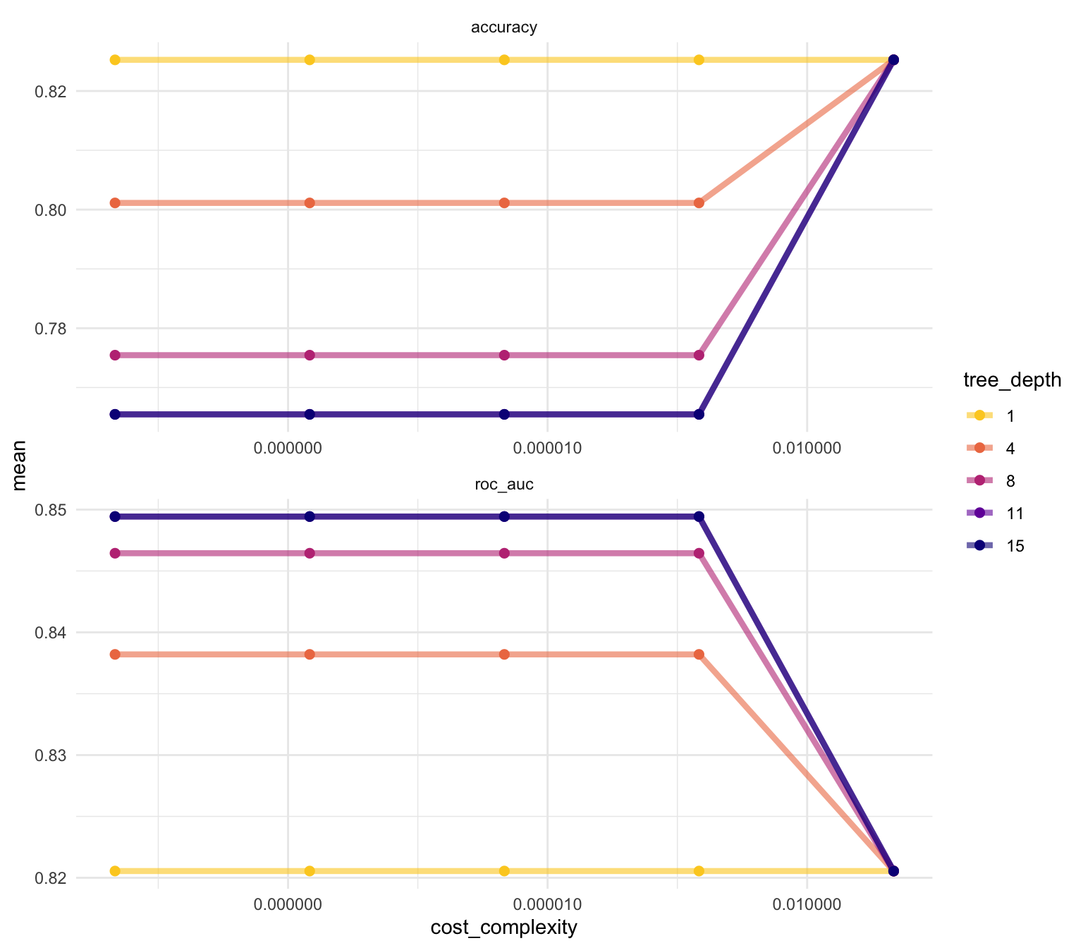
We can see that our “stubbiest” tree, with a depth of 1, is the worst model according to roc_auc (though surprisingly the most accurate) and across all candidate values of cost_complexity. Deeper trees tend to do better for this problem. However, the best tree seems to be between these values with a tree depth of 8. The show_best() function shows us the top 5 candidate models by default:
tree_res %>%
  show_best("roc_auc")
## # A tibble: 5 × 8
##   cost_complexity tree_depth .metric .estimator  mean     n std_err .config
##             <dbl>      <int> <chr>   <chr>      <dbl> <int>   <dbl> <chr>
## 1    0.0000000001         11 roc_auc binary     0.849    10  0.0171 Preprocesso…
## 2    0.0000000178         11 roc_auc binary     0.849    10  0.0171 Preprocesso…
## 3    0.00000316           11 roc_auc binary     0.849    10  0.0171 Preprocesso…
## 4    0.000562             11 roc_auc binary     0.849    10  0.0171 Preprocesso…
## 5    0.0000000001         15 roc_auc binary     0.849    10  0.0171 Preprocesso…
We can also use the select_best() function to pull out the single set of hyperparameter values for our best decision tree model:
best_tree <- tree_res %>%
  select_best("roc_auc")

best_tree
## # A tibble: 1 × 3
##   cost_complexity tree_depth .config
##             <dbl>      <int> <chr>
## 1    0.0000000001         11 Preprocessor1_Model16
These are the values for tree_depth and cost_complexity that maximize AUC in this data set of respondents.
Finalizing our model
We can update (or “finalize”) our workflow object tree_wf with the values from select_best().
final_wf <-
  tree_wf %>%
  finalize_workflow(best_tree)

final_wf
## ══ Workflow ════════════════════════════════════════════════════════════════════
## Preprocessor: Formula
## Model: decision_tree()
##
## ── Preprocessor ────────────────────────────────────────────────────────────────
## colmslm ~ .
##
## ── Model ───────────────────────────────────────────────────────────────────────
## Decision Tree Model Specification (classification)
##
## Main Arguments:
##   cost_complexity = 1e-10
##   tree_depth = 11
##
## Computational engine: rpart
Our tuning is done!
Exploring results
Let’s fit this final model to the training data. What does the decision tree look like?
final_tree <-
  final_wf %>%
  fit(data = gss_train)

final_tree
## ══ Workflow [trained] ══════════════════════════════════════════════════════════
## Preprocessor: Formula
## Model: decision_tree()
##
## ── Preprocessor ────────────────────────────────────────────────────────────────
## colmslm ~ .
##
## ── Model ───────────────────────────────────────────────────────────────────────
## n= 704
##
## node), split, n, loss, yval, (yprob)
##       * denotes terminal node
##
##    1) root 704 268 Not allowed (0.38068182 0.61931818)
##      2) tolerance>=12.5 289  72 Yes, allowed (0.75086505 0.24913495)
##        4) tolerance>=13.5 227  43 Yes, allowed (0.81057269 0.18942731)
##          8) id< 463 53   2 Yes, allowed (0.96226415 0.03773585) *
##          9) id>=463 174  41 Yes, allowed (0.76436782 0.23563218)
##           18) id>=595.5 156  32 Yes, allowed (0.79487179 0.20512821)
##             36) pray=SEVERAL TIMES A DAY,SEVERAL TIMES A WEEK,ONCE A WEEK 61   5 Yes, allowed (0.91803279 0.08196721) *
##             37) pray=ONCE A DAY,LT ONCE A WEEK,NEVER 95  27 Yes, allowed (0.71578947 0.28421053)
##               74) id< 1841.5 85  21 Yes, allowed (0.75294118 0.24705882)
##                148) id< 705.5 8   0 Yes, allowed (1.00000000 0.00000000) *
##                149) id>=705.5 77  21 Yes, allowed (0.72727273 0.27272727)
##                  298) wtss>=1.441643 13   1 Yes, allowed (0.92307692 0.07692308) *
##                  299) wtss< 1.441643 64  20 Yes, allowed (0.68750000 0.31250000)
##                    598) age>=67.5 10   1 Yes, allowed (0.90000000 0.10000000) *
##                    599) age< 67.5 54  19 Yes, allowed (0.64814815 0.35185185)
##                     1198) age< 50.5 37  10 Yes, allowed (0.72972973 0.27027027) *
##                     1199) age>=50.5 17   8 Not allowed (0.47058824 0.52941176) *
##               75) id>=1841.5 10   4 Not allowed (0.40000000 0.60000000) *
##           19) id< 595.5 18   9 Yes, allowed (0.50000000 0.50000000) *
##        5) tolerance< 13.5 62  29 Yes, allowed (0.53225806 0.46774194)
##         10) pray=SEVERAL TIMES A DAY,ONCE A DAY,SEVERAL TIMES A WEEK,LT ONCE A WEEK 47  17 Yes, allowed (0.63829787 0.36170213)
##           20) polviews=ExtrmLib,Moderate,SlghtCons,ExtrmCons 30   7 Yes, allowed (0.76666667 0.23333333) *
##           21) polviews=Liberal,SlghtLib,Conserv 17   7 Not allowed (0.41176471 0.58823529) *
##         11) pray=ONCE A WEEK,NEVER 15   3 Not allowed (0.20000000 0.80000000) *
##      3) tolerance< 12.5 415  51 Not allowed (0.12289157 0.87710843)
##        6) id< 641 121  27 Not allowed (0.22314050 0.77685950)
##         12) tolerance>=7.5 86  27 Not allowed (0.31395349 0.68604651)
##           24) id>=575 7   1 Yes, allowed (0.85714286 0.14285714) *
##           25) id< 575 79  21 Not allowed (0.26582278 0.73417722)
##             50) pray=SEVERAL TIMES A DAY,NEVER 32  13 Not allowed (0.40625000 0.59375000)
##              100) degree=<HS,Graduate deg 7   1 Yes, allowed (0.85714286 0.14285714) *
##              101) degree=HS,Junior Coll,Bachelor deg 25   7 Not allowed (0.28000000 0.72000000)
##                202) id< 218 7   3 Yes, allowed (0.57142857 0.42857143) *
##                203) id>=218 18   3 Not allowed (0.16666667 0.83333333) *
##             51) pray=ONCE A DAY,SEVERAL TIMES A WEEK,ONCE A WEEK,LT ONCE A WEEK 47   8 Not allowed (0.17021277 0.82978723) *
##         13) tolerance< 7.5 35   0 Not allowed (0.00000000 1.00000000) *
##        7) id>=641 294  24 Not allowed (0.08163265 0.91836735) *
This final_tree object has the finalized, fitted model object inside. You may want to extract the model object from the workflow. To do this, you can use the helper function pull_workflow_fit().
For example, perhaps we would also like to understand what variables are important in this final model. We can use the vip package to estimate variable importance.
library(vip)

final_tree %>%
  pull_workflow_fit() %>%
  vip()
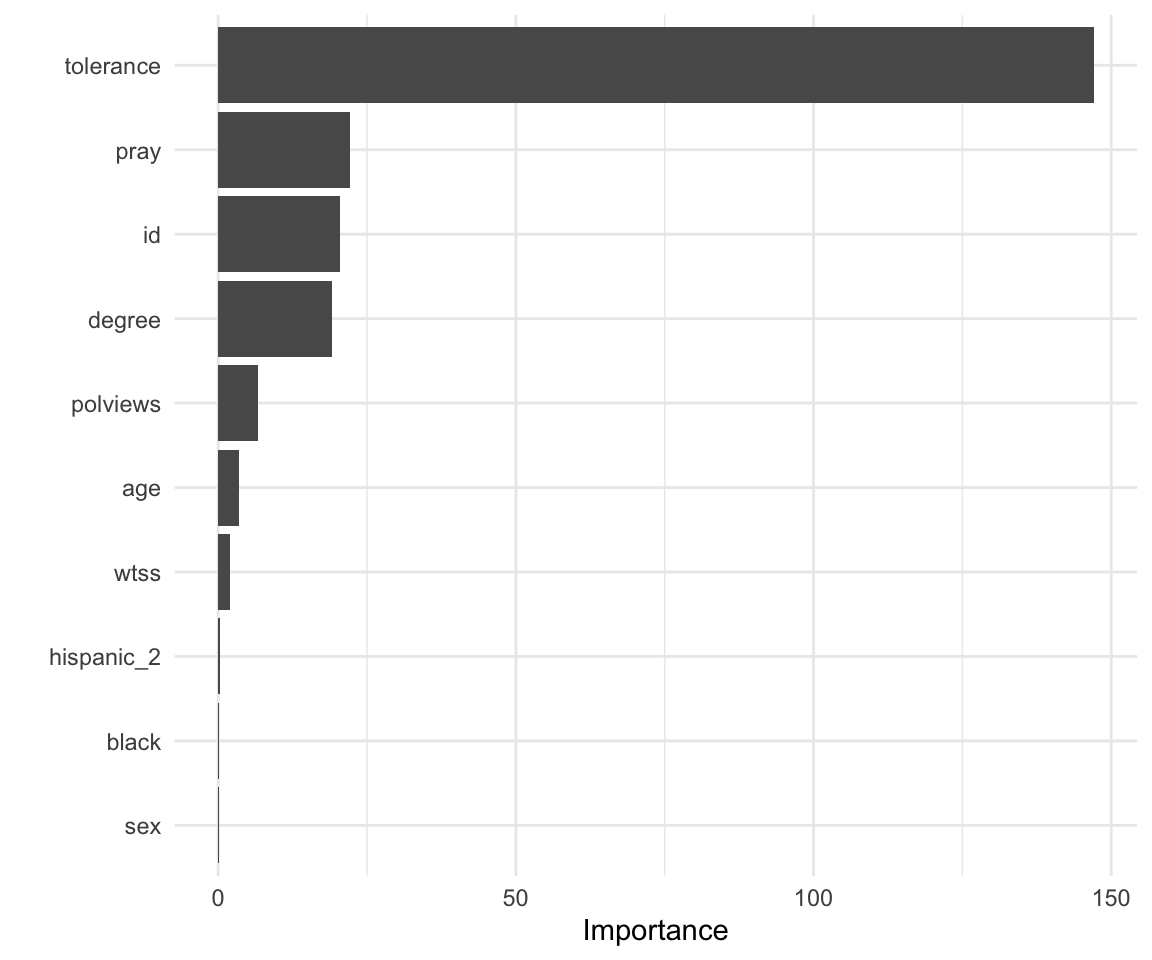
These are the survey variables that are the most important in driving predictions on the Muslim clergymen question.
The last fit
Finally, let’s return to our test data and estimate the model performance we expect to see with new data. We can use the function last_fit() with our finalized model; this function fits the finalized model on the full training data set and evaluates the finalized model on the testing data.
final_fit <-
  final_wf %>%
  last_fit(gss_split)

final_fit %>%
  collect_metrics()
## # A tibble: 2 × 4
##   .metric  .estimator .estimate .config
##   <chr>    <chr>          <dbl> <chr>
## 1 accuracy binary         0.771 Preprocessor1_Model1
## 2 roc_auc  binary         0.811 Preprocessor1_Model1
final_fit %>%
  collect_predictions() %>%
  roc_curve(colmslm, `.pred_Yes, allowed`) %>%
  autoplot()
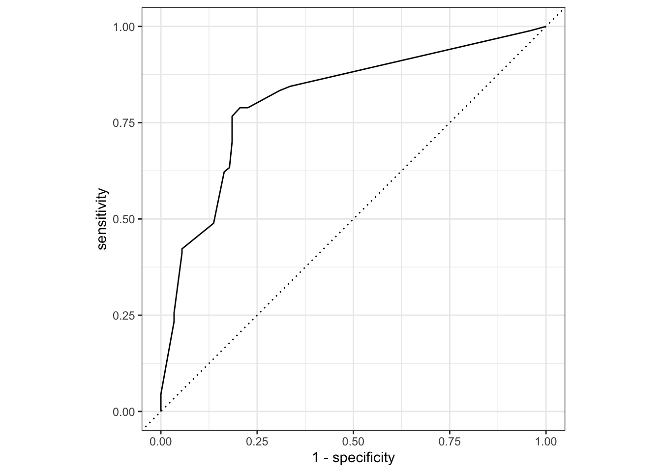
The performance metrics from the test set indicate that we did not overfit during our tuning procedure.
We leave it to the reader to explore whether you can tune a different decision tree hyperparameter. You can explore the reference docs, or use the args() function to see which parsnip object arguments are available:
args(decision_tree)
## function (mode = "unknown", engine = "rpart", cost_complexity = NULL,
##     tree_depth = NULL, min_n = NULL)
## NULL
You could tune the other hyperparameter we didn’t use here, min_n, which sets the minimum n to split at any node. This is another early stopping method for decision trees that can help prevent overfitting. Use this searchable table to find the original argument for min_n in the rpart package (hint). See whether you can tune a different combination of hyperparameters and/or values to improve a tree’s ability to predict respondents’ answers.
Acknowledgments
Example drawn from Get Started - Tune model parameters and licensed under CC BY-SA 4.0.
Session Info
sessioninfo::session_info()
## ─ Session info ───────────────────────────────────────────────────────────────
##  setting  value
##  version  R version 4.2.1 (2022-06-23)
##  os       macOS Monterey 12.3
##  system   aarch64, darwin20
##  ui       X11
##  language (EN)
##  collate  en_US.UTF-8
##  ctype    en_US.UTF-8
##  tz       America/New_York
##  date     2022-08-22
##  pandoc   2.18 @ /Applications/RStudio.app/Contents/MacOS/quarto/bin/tools/ (via rmarkdown)
##
## ─ Packages ───────────────────────────────────────────────────────────────────
##  package      * version    date (UTC) lib source
##  assertthat     0.2.1      2019-03-21 [2] CRAN (R 4.2.0)
##  backports      1.4.1      2021-12-13 [2] CRAN (R 4.2.0)
##  blogdown       1.10       2022-05-10 [2] CRAN (R 4.2.0)
##  bookdown       0.27       2022-06-14 [2] CRAN (R 4.2.0)
##  broom        * 1.0.0      2022-07-01 [2] CRAN (R 4.2.0)
##  bslib          0.4.0      2022-07-16 [2] CRAN (R 4.2.0)
##  cachem         1.0.6      2021-08-19 [2] CRAN (R 4.2.0)
##  class          7.3-20     2022-01-16 [2] CRAN (R 4.2.1)
##  cli            3.3.0      2022-04-25 [2] CRAN (R 4.2.0)
##  codetools      0.2-18     2020-11-04 [2] CRAN (R 4.2.1)
##  colorspace     2.0-3      2022-02-21 [2] CRAN (R 4.2.0)
##  DBI            1.1.3      2022-06-18 [2] CRAN (R 4.2.0)
##  dials        * 1.0.0      2022-06-14 [2] CRAN (R 4.2.0)
##  DiceDesign     1.9        2021-02-13 [2] CRAN (R 4.2.0)
##  digest         0.6.29     2021-12-01 [2] CRAN (R 4.2.0)
##  doParallel     1.0.17     2022-02-07 [2] CRAN (R 4.2.0)
##  dplyr        * 1.0.9      2022-04-28 [2] CRAN (R 4.2.0)
##  evaluate       0.16       2022-08-09 [1] CRAN (R 4.2.1)
##  fansi          1.0.3      2022-03-24 [2] CRAN (R 4.2.0)
##  fastmap        1.1.0      2021-01-25 [2] CRAN (R 4.2.0)
##  foreach        1.5.2      2022-02-02 [2] CRAN (R 4.2.0)
##  furrr          0.3.0      2022-05-04 [2] CRAN (R 4.2.0)
##  future         1.27.0     2022-07-22 [2] CRAN (R 4.2.0)
##  future.apply   1.9.0      2022-04-25 [2] CRAN (R 4.2.0)
##  generics       0.1.3      2022-07-05 [2] CRAN (R 4.2.0)
##  ggplot2      * 3.3.6      2022-05-03 [2] CRAN (R 4.2.0)
##  globals        0.16.0     2022-08-05 [2] CRAN (R 4.2.0)
##  glue           1.6.2      2022-02-24 [2] CRAN (R 4.2.0)
##  gower          1.0.0      2022-02-03 [2] CRAN (R 4.2.0)
##  GPfit          1.0-8      2019-02-08 [2] CRAN (R 4.2.0)
##  gridExtra      2.3        2017-09-09 [2] CRAN (R 4.2.0)
##  gtable         0.3.0      2019-03-25 [2] CRAN (R 4.2.0)
##  hardhat        1.2.0      2022-06-30 [2] CRAN (R 4.2.0)
##  here           1.0.1      2020-12-13 [2] CRAN (R 4.2.0)
##  htmltools      0.5.3      2022-07-18 [2] CRAN (R 4.2.0)
##  httr           1.4.3      2022-05-04 [2] CRAN (R 4.2.0)
##  infer        * 1.0.2      2022-06-10 [2] CRAN (R 4.2.0)
##  ipred          0.9-13     2022-06-02 [2] CRAN (R 4.2.0)
##  iterators      1.0.14     2022-02-05 [2] CRAN (R 4.2.0)
##  jquerylib      0.1.4      2021-04-26 [2] CRAN (R 4.2.0)
##  jsonlite       1.8.0      2022-02-22 [2] CRAN (R 4.2.0)
##  kableExtra   * 1.3.4      2021-02-20 [2] CRAN (R 4.2.0)
##  knitr          1.39       2022-04-26 [2] CRAN (R 4.2.0)
##  lattice        0.20-45    2021-09-22 [2] CRAN (R 4.2.1)
##  lava           1.6.10     2021-09-02 [2] CRAN (R 4.2.0)
##  lhs            1.1.5      2022-03-22 [2] CRAN (R 4.2.0)
##  lifecycle      1.0.1      2021-09-24 [2] CRAN (R 4.2.0)
##  listenv        0.8.0      2019-12-05 [2] CRAN (R 4.2.0)
##  lubridate      1.8.0      2021-10-07 [2] CRAN (R 4.2.0)
##  magrittr       2.0.3      2022-03-30 [2] CRAN (R 4.2.0)
##  MASS           7.3-58.1   2022-08-03 [2] CRAN (R 4.2.0)
##  Matrix         1.4-1      2022-03-23 [2] CRAN (R 4.2.1)
##  modeldata    * 1.0.0      2022-07-01 [2] CRAN (R 4.2.0)
##  munsell        0.5.0      2018-06-12 [2] CRAN (R 4.2.0)
##  nnet           7.3-17     2022-01-16 [2] CRAN (R 4.2.1)
##  parallelly     1.32.1     2022-07-21 [2] CRAN (R 4.2.0)
##  parsnip      * 1.0.0      2022-06-16 [2] CRAN (R 4.2.0)
##  pillar         1.8.0      2022-07-18 [2] CRAN (R 4.2.0)
##  pkgconfig      2.0.3      2019-09-22 [2] CRAN (R 4.2.0)
##  prodlim        2019.11.13 2019-11-17 [2] CRAN (R 4.2.0)
##  purrr        * 0.3.4      2020-04-17 [2] CRAN (R 4.2.0)
##  R6             2.5.1      2021-08-19 [2] CRAN (R 4.2.0)
##  Rcpp           1.0.9      2022-07-08 [2] CRAN (R 4.2.0)
##  recipes      * 1.0.1      2022-07-07 [2] CRAN (R 4.2.0)
##  rlang          1.0.4      2022-07-12 [2] CRAN (R 4.2.0)
##  rmarkdown      2.14       2022-04-25 [2] CRAN (R 4.2.0)
##  rpart        * 4.1.16     2022-01-24 [2] CRAN (R 4.2.1)
##  rprojroot      2.0.3      2022-04-02 [2] CRAN (R 4.2.0)
##  rsample      * 1.1.0      2022-08-08 [2] CRAN (R 4.2.1)
##  rstudioapi     0.13       2020-11-12 [2] CRAN (R 4.2.0)
##  rvest          1.0.2      2021-10-16 [2] CRAN (R 4.2.0)
##  sass           0.4.2      2022-07-16 [2] CRAN (R 4.2.0)
##  scales       * 1.2.0      2022-04-13 [2] CRAN (R 4.2.0)
##  sessioninfo    1.2.2      2021-12-06 [2] CRAN (R 4.2.0)
##  stringi        1.7.8      2022-07-11 [2] CRAN (R 4.2.0)
##  stringr        1.4.0      2019-02-10 [2] CRAN (R 4.2.0)
##  survival       3.3-1      2022-03-03 [2] CRAN (R 4.2.1)
##  svglite        2.1.0      2022-02-03 [2] CRAN (R 4.2.0)
##  systemfonts    1.0.4      2022-02-11 [2] CRAN (R 4.2.0)
##  tibble       * 3.1.8      2022-07-22 [2] CRAN (R 4.2.0)
##  tidymodels   * 1.0.0      2022-07-13 [2] CRAN (R 4.2.0)
##  tidyr        * 1.2.0      2022-02-01 [2] CRAN (R 4.2.0)
##  tidyselect     1.1.2      2022-02-21 [2] CRAN (R 4.2.0)
##  timeDate       4021.104   2022-07-19 [2] CRAN (R 4.2.0)
##  tune         * 1.0.0      2022-07-07 [2] CRAN (R 4.2.0)
##  utf8           1.2.2      2021-07-24 [2] CRAN (R 4.2.0)
##  vctrs          0.4.1      2022-04-13 [2] CRAN (R 4.2.0)
##  vip          * 0.3.2      2020-12-17 [2] CRAN (R 4.2.0)
##  viridisLite    0.4.0      2021-04-13 [2] CRAN (R 4.2.0)
##  webshot        0.5.3      2022-04-14 [2] CRAN (R 4.2.0)
##  withr          2.5.0      2022-03-03 [2] CRAN (R 4.2.0)
##  workflows    * 1.0.0      2022-07-05 [2] CRAN (R 4.2.0)
##  workflowsets * 1.0.0      2022-07-12 [2] CRAN (R 4.2.0)
##  xfun           0.31       2022-05-10 [1] CRAN (R 4.2.0)
##  xml2           1.3.3      2021-11-30 [2] CRAN (R 4.2.0)
##  yaml           2.3.5      2022-02-21 [2] CRAN (R 4.2.0)
##  yardstick    * 1.0.0      2022-06-06 [2] CRAN (R 4.2.0)
##
##  [1] /Users/soltoffbc/Library/R/arm64/4.2/library
##  [2] /Library/Frameworks/R.framework/Versions/4.2-arm64/Resources/library
##
## ──────────────────────────────────────────────────────────────────────────────