Build a linear model
library(tidymodels)
library(tidyverse)
library(rcis)
library(rstanarm)
library(broom.mixed)

set.seed(123)
theme_set(theme_minimal())
Introduction
There are several different approaches to fitting a linear model in R.1 Here, we introduce tidymodels and demonstrate how to construct a basic linear regression model.
tidymodels is a collection of packages for statistical modeling and machine learning using tidyverse principles. Given this emphasis, it pairs nicely with the tidy-centric approach we have covered so far for tasks such as data visualization, data wrangling, importation of data files, and publishing results.
tidymodels is still under active development and contains a range of packages and functions for many different aspects of statistical modeling. Here we demonstrate how to start with data for modeling, specify and train models using different engines using the parsnip package, and understand why these functions are designed this way.
scorecard
As in past exercises, let’s use the rcis::scorecard dataset which contains detailed information on all four-year colleges and universities in the United States. Here we will consider the average faculty salary to understand how it is influenced by factors such as the average annual total cost of attendance and whether the university is public, private nonprofit, or private for-profit.
scorecard
## # A tibble: 1,732 × 14
## unitid name state type admrate satavg cost netcost avgfa…¹ pctpell compr…²
## <dbl> <chr> <chr> <fct> <dbl> <dbl> <dbl> <dbl> <dbl> <dbl> <dbl>
## 1 100654 Alab… AL Publ… 0.918 939 23053 14990 69381 0.702 0.297
## 2 100663 Univ… AL Publ… 0.737 1234 24495 16953 99441 0.351 0.634
## 3 100706 Univ… AL Publ… 0.826 1319 23917 15860 87192 0.254 0.577
## 4 100724 Alab… AL Publ… 0.969 946 21866 13650 64989 0.763 0.328
## 5 100751 The … AL Publ… 0.827 1261 29872 22597 92619 0.177 0.711
## 6 100830 Aubu… AL Publ… 0.904 1082 19849 13987 71343 0.464 0.340
## 7 100858 Aubu… AL Publ… 0.807 1300 31590 24104 96642 0.146 0.791
## 8 100937 Birm… AL Priv… 0.538 1230 32095 22107 56646 0.236 0.691
## 9 101189 Faul… AL Priv… 0.783 1066 34317 20715 54009 0.488 0.329
## 10 101365 Herz… AL Priv… 0.783 NA 30119 26680 54684 0.706 0.28
## # … with 1,722 more rows, 3 more variables: firstgen <dbl>, debt <dbl>,
## # locale <fct>, and abbreviated variable names ¹avgfacsal, ²comprate
## # ℹ Use `print(n = ...)` to see more rows, and `colnames()` to see all variable names
glimpse(scorecard)
## Rows: 1,732
## Columns: 14
## $ unitid    <dbl> 100654, 100663, 100706, 100724, 100751, 100830, 100858, 1009…
## $ name      <chr> "Alabama A & M University", "University of Alabama at Birmin…
## $ state     <chr> "AL", "AL", "AL", "AL", "AL", "AL", "AL", "AL", "AL", "AL", …
## $ type      <fct> "Public", "Public", "Public", "Public", "Public", "Public", …
## $ admrate   <dbl> 0.9175, 0.7366, 0.8257, 0.9690, 0.8268, 0.9044, 0.8067, 0.53…
## $ satavg    <dbl> 939, 1234, 1319, 946, 1261, 1082, 1300, 1230, 1066, NA, 1076…
## $ cost      <dbl> 23053, 24495, 23917, 21866, 29872, 19849, 31590, 32095, 3431…
## $ netcost   <dbl> 14990, 16953, 15860, 13650, 22597, 13987, 24104, 22107, 2071…
## $ avgfacsal <dbl> 69381, 99441, 87192, 64989, 92619, 71343, 96642, 56646, 5400…
## $ pctpell   <dbl> 0.7019, 0.3512, 0.2536, 0.7627, 0.1772, 0.4644, 0.1455, 0.23…
## $ comprate  <dbl> 0.2974, 0.6340, 0.5768, 0.3276, 0.7110, 0.3401, 0.7911, 0.69…
## $ firstgen  <dbl> 0.3658281, 0.3412237, 0.3101322, 0.3434343, 0.2257127, 0.381…
## $ debt      <dbl> 15250, 15085, 14000, 17500, 17671, 12000, 17500, 16000, 1425…
## $ locale    <fct> City, City, City, City, City, City, City, City, City, Suburb…
As a first step in modeling, it’s always a good idea to plot the data:
ggplot(
  data = scorecard,
  mapping = aes(
    x = cost,
    y = avgfacsal,
    col = type
  )
) +
  geom_point(alpha = .3) +
  geom_smooth(method = lm, se = FALSE) +
  scale_color_viridis_d(option = "plasma", end = .7)
## `geom_smooth()` using formula 'y ~ x'
## Warning: Removed 62 rows containing non-finite values (stat_smooth).
## Warning: Removed 62 rows containing missing values (geom_point).
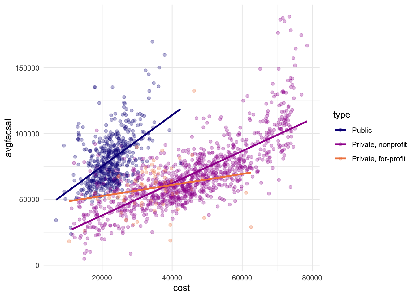
We can see that public and private non-profit schools have the strongest correlation between total cost of attendance and average faculty salaries – private for-profit schools tend to be pretty flat in terms of average salaries regardless of cost of attendance.
Build and fit a model
A standard two-way analysis of variance (ANOVA) model makes sense for this dataset because we have both a continuous predictor and a categorical predictor. Since the slopes appear to be different for at least two of the college types, let’s build a model that allows for two-way interactions. Specifying an R formula with our variables in this way:
avgfacsal ~ cost * type
allows our regression model depending on cost to have separate slopes and intercepts for each type of college.
For this kind of model, ordinary least squares is a good initial approach. With tidymodels, we start by specifying the functional form of the model that we want using the parsnip package. Since there is a numeric outcome and the model should be linear with slopes and intercepts, the model type is “linear regression”. We can declare this with:
linear_reg()
## Linear Regression Model Specification (regression)
##
## Computational engine: lm
That is pretty underwhelming since, on its own, it doesn’t really do much. However, now that the type of model has been specified, a method for fitting or training the model can be stated using the engine. The engine value is often a mash-up of the software that can be used to fit or train the model as well as the estimation method. For example, to use ordinary least squares, we can set the engine to be lm:
linear_reg() %>%
  set_engine("lm")
## Linear Regression Model Specification (regression)
##
## Computational engine: lm
The documentation page for linear_reg() lists the possible engines. We’ll save this model object as lm_mod.
lm_mod <- linear_reg() %>%
  set_engine("lm")
From here, the model can be estimated or trained using the fit() function:
lm_fit <- lm_mod %>%
  fit(avgfacsal ~ cost * type, data = scorecard)
lm_fit
## parsnip model object
##
##
## Call:
## stats::lm(formula = avgfacsal ~ cost * type, data = data)
##
## Coefficients:
##                  (Intercept)                          cost
##                    3.629e+04                     1.944e+00
##       typePrivate, nonprofit       typePrivate, for-profit
##                   -2.291e+04                     7.919e+03
##  cost:typePrivate, nonprofit  cost:typePrivate, for-profit
##                   -7.219e-01                    -1.525e+00
Perhaps our analysis requires a description of the model parameter estimates and their statistical properties. Although the summary() function for lm objects can provide that, it gives the results back in an unwieldy format. Many models have a tidy() method that provides the summary results in a more predictable and useful format (e.g. a data frame with standard column names):
tidy(lm_fit)
## # A tibble: 6 × 5
##   term                           estimate std.error statistic  p.value
##   <chr>                             <dbl>     <dbl>     <dbl>    <dbl>
## 1 (Intercept)                   36286.     3288.       11.0   2.21e-27
## 2 cost                              1.94      0.143    13.6   4.55e-40
## 3 typePrivate, nonprofit       -22913.     3623.       -6.32  3.25e-10
## 4 typePrivate, for-profit        7919.     8229.        0.962 3.36e- 1
## 5 cost:typePrivate, nonprofit      -0.722     0.146    -4.93  8.95e- 7
## 6 cost:typePrivate, for-profit     -1.53      0.260    -5.87  5.28e- 9
Use a model to predict
This fitted object lm_fit has the lm model output built-in, which you can access with lm_fit$fit, but there are some benefits to using the fitted parsnip model object when it comes to predicting.
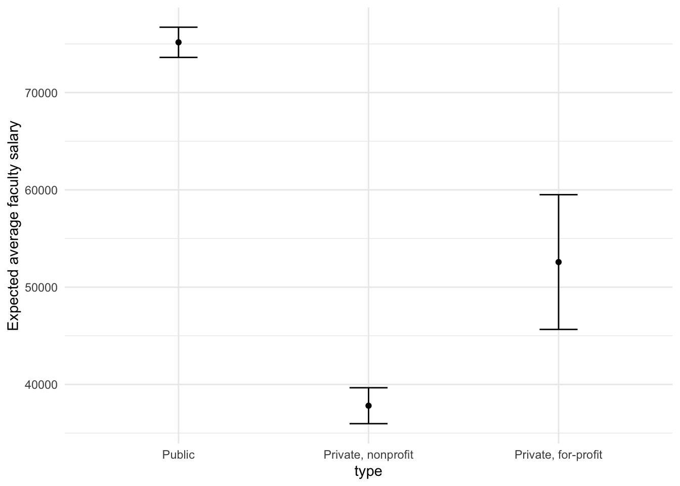
Suppose that, for a publication, it would be particularly interesting to make a plot of the expected average faculty salary for colleges with a total cost of attendance of $20,000. To create such a graph, we start with some new example data that we will make predictions for, to show in our graph:
new_points <- expand.grid(
  cost = 20000,
  type = c("Public", "Private, nonprofit", "Private, for-profit")
)
new_points
##    cost                type
## 1 20000              Public
## 2 20000  Private, nonprofit
## 3 20000 Private, for-profit
To get our predicted results, we can use the predict() function to find the expected salaries at $20,000 cost of attendance.
It is also important to communicate the variability, so we also need to find the predicted confidence intervals. If we had used lm() to fit the model directly, a few minutes of reading the documentation page for predict.lm() would explain how to do this. However, if we decide to use a different model to estimate average faculty salaries (spoiler: we will!), it is likely that a completely different syntax would be required.
Instead, with tidymodels, the types of predicted values are standardized so that we can use the same syntax to get these values.
First, let’s generate the expected salary values:
mean_pred <- predict(lm_fit, new_data = new_points)
mean_pred
## # A tibble: 3 × 1
##    .pred
##    <dbl>
## 1 75167.
## 2 37816.
## 3 52580.
When making predictions, the tidymodels convention is to always produce a tibble of results with standardized column names. This makes it easy to combine the original data and the predictions in a usable format:
conf_int_pred <- predict(lm_fit,
  new_data = new_points,
  type = "conf_int"
)
conf_int_pred
## # A tibble: 3 × 2
##   .pred_lower .pred_upper
##         <dbl>       <dbl>
## 1      73618.      76717.
## 2      35970.      39662.
## 3      45656.      59504.
# Now combine
plot_data <- new_points %>%
  bind_cols(mean_pred) %>%
  bind_cols(conf_int_pred)

# And plot
ggplot(data = plot_data, mapping = aes(x = type)) +
  geom_point(mapping = aes(y = .pred)) +
  geom_errorbar(
    mapping = aes(
      ymin = .pred_lower,
      ymax = .pred_upper
    ),
    width = .2
  ) +
  labs(y = "Expected average faculty salary")
Model with a different engine
Every one on your team is happy with that plot except that one person who just read their first book on Bayesian analysis. They are interested in knowing if the results would be different if the model were estimated using a Bayesian approach. In such an analysis, a prior distribution needs to be declared for each model parameter that represents the possible values of the parameters (before being exposed to the observed data). After some discussion, the group agrees that the priors should be bell-shaped but, since no one has any idea what the range of values should be, to take a conservative approach and make the priors wide using a Cauchy distribution (which is the same as a t-distribution with a single degree of freedom).
The documentation on the rstanarm package shows us that the stan_glm() function can be used to estimate this model, and that the function arguments that need to be specified are called prior and prior_intercept. It turns out that linear_reg() has a stan engine. Since these prior distribution arguments are specific to the Stan software, they are passed as arguments to parsnip::set_engine(). After that, the same exact fit() call is used:
# set the prior distribution
prior_dist <- rstanarm::student_t(df = 1)

set.seed(123)

# make the parsnip model
bayes_mod <- linear_reg() %>%
  set_engine("stan",
    prior_intercept = prior_dist,
    prior = prior_dist,
    # increase number of iterations to converge to stable solution
    iter = 4000
  )

# train the model
bayes_fit <- bayes_mod %>%
  fit(avgfacsal ~ cost * type, data = scorecard)

print(bayes_fit, digits = 5)
## parsnip model object
##
## stan_glm
##  family:       gaussian [identity]
##  formula:      avgfacsal ~ cost * type
##  observations: 1670
##  predictors:   6
## ------
##                              Median       MAD_SD
## (Intercept)                   34364.69103   4847.98681
## cost                              2.02604      0.21169
## typePrivate, nonprofit       -20327.03309   5481.34882
## typePrivate, for-profit           0.06524      3.69244
## cost:typePrivate, nonprofit      -0.81531      0.21867
## cost:typePrivate, for-profit     -1.34440      0.11960
##
## Auxiliary parameter(s):
##       Median      MAD_SD
## sigma 16324.73848   302.10087
##
## ------
## * For help interpreting the printed output see ?print.stanreg
## * For info on the priors used see ?prior_summary.stanreg
set.seed() to ensure that the same (pseudo-)random numbers are generated each time we run this code. The number 123 isn’t special or related to our data; it is just a “seed” used to choose random numbers.To update the parameter table, the tidy() method is once again used:
tidy(bayes_fit, conf.int = TRUE)
## # A tibble: 6 × 5
##   term                            estimate std.error  conf.low conf.high
##   <chr>                              <dbl>     <dbl>     <dbl>     <dbl>
## 1 (Intercept)                   34365.      4848.     17250.   40410.
## 2 cost                              2.03       0.212      1.76     2.76
## 3 typePrivate, nonprofit       -20327.      5481.    -27061.       3.50
## 4 typePrivate, for-profit           0.0652     3.69     -15.3     15.5
## 5 cost:typePrivate, nonprofit      -0.815      0.219     -1.62    -0.546
## 6 cost:typePrivate, for-profit     -1.34       0.120     -1.62    -1.19
A goal of the tidymodels packages is that the interfaces to common tasks are standardized (as seen in the tidy() results above). The same is true for getting predictions; we can use the same code even though the underlying packages use very different syntax:
bayes_plot_data <- new_points %>%
  bind_cols(predict(bayes_fit, new_data = new_points)) %>%
  bind_cols(predict(bayes_fit, new_data = new_points, type = "conf_int"))

ggplot(data = bayes_plot_data, mapping = aes(x = type)) +
  geom_point(mapping = aes(y = .pred)) +
  geom_errorbar(
    mapping = aes(
      ymin = .pred_lower,
      ymax = .pred_upper
    ),
    width = .2
  ) +
  labs(y = "Expected average faculty salary")
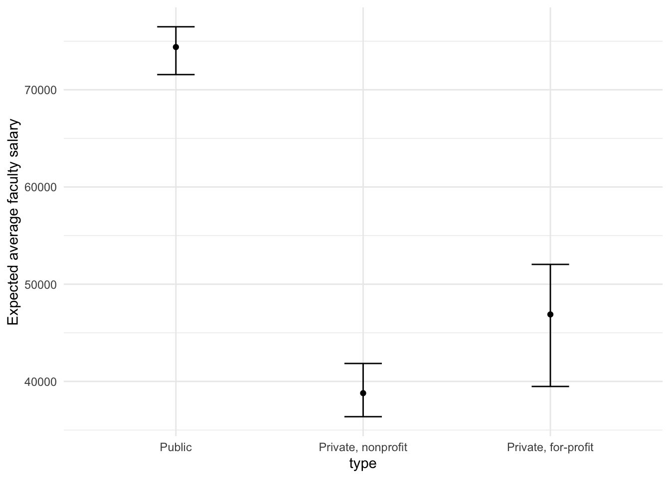
This isn’t very different from the non-Bayesian results (except in interpretation).
parsnip package can work with many model types, engines, and arguments. Check out tidymodels.org/find/parsnip/ to see what is available.Why does it work that way?
The extra step of defining the model using a function like linear_reg() might seem superfluous since a call to lm() is much more succinct. However, the problem with standard modeling functions is that they don’t separate what you want to do from the execution. For example, the process of executing a formula has to happen repeatedly across model calls even when the formula does not change; we can’t recycle those computations.
Also, using the tidymodels framework, we can do some interesting things by incrementally creating a model (instead of using single function call). Model tuning with tidymodels uses the specification of the model to declare what parts of the model should be tuned. That would be very difficult to do if linear_reg() immediately fit the model.
Acknowledgments
- Example drawn from Get Started - Build a model and licensed under CC BY-SA 4.0.
- Artwork by @allison_horst
Session Info
sessioninfo::session_info()
## ─ Session info ───────────────────────────────────────────────────────────────
##  setting  value
##  version  R version 4.2.1 (2022-06-23)
##  os       macOS Monterey 12.3
##  system   aarch64, darwin20
##  ui       X11
##  language (EN)
##  collate  en_US.UTF-8
##  ctype    en_US.UTF-8
##  tz       America/New_York
##  date     2022-08-22
##  pandoc   2.18 @ /Applications/RStudio.app/Contents/MacOS/quarto/bin/tools/ (via rmarkdown)
##
## ─ Packages ───────────────────────────────────────────────────────────────────
##  package       * version    date (UTC) lib source
##  assertthat      0.2.1      2019-03-21 [2] CRAN (R 4.2.0)
##  backports       1.4.1      2021-12-13 [2] CRAN (R 4.2.0)
##  base64enc       0.1-3      2015-07-28 [2] CRAN (R 4.2.0)
##  bayesplot       1.9.0      2022-03-10 [2] CRAN (R 4.2.0)
##  blogdown        1.10       2022-05-10 [2] CRAN (R 4.2.0)
##  bookdown        0.27       2022-06-14 [2] CRAN (R 4.2.0)
##  boot            1.3-28     2021-05-03 [2] CRAN (R 4.2.1)
##  broom         * 1.0.0      2022-07-01 [2] CRAN (R 4.2.0)
##  broom.mixed   * 0.2.9.4    2022-04-17 [2] CRAN (R 4.2.0)
##  bslib           0.4.0      2022-07-16 [2] CRAN (R 4.2.0)
##  cachem          1.0.6      2021-08-19 [2] CRAN (R 4.2.0)
##  callr           3.7.1      2022-07-13 [2] CRAN (R 4.2.0)
##  cellranger      1.1.0      2016-07-27 [2] CRAN (R 4.2.0)
##  class           7.3-20     2022-01-16 [2] CRAN (R 4.2.1)
##  cli             3.3.0      2022-04-25 [2] CRAN (R 4.2.0)
##  codetools       0.2-18     2020-11-04 [2] CRAN (R 4.2.1)
##  colorspace      2.0-3      2022-02-21 [2] CRAN (R 4.2.0)
##  colourpicker    1.1.1      2021-10-04 [2] CRAN (R 4.2.0)
##  crayon          1.5.1      2022-03-26 [2] CRAN (R 4.2.0)
##  crosstalk       1.2.0      2021-11-04 [2] CRAN (R 4.2.0)
##  DBI             1.1.3      2022-06-18 [2] CRAN (R 4.2.0)
##  dbplyr          2.2.1      2022-06-27 [2] CRAN (R 4.2.0)
##  dials         * 1.0.0      2022-06-14 [2] CRAN (R 4.2.0)
##  DiceDesign      1.9        2021-02-13 [2] CRAN (R 4.2.0)
##  digest          0.6.29     2021-12-01 [2] CRAN (R 4.2.0)
##  dplyr         * 1.0.9      2022-04-28 [2] CRAN (R 4.2.0)
##  DT              0.23       2022-05-10 [2] CRAN (R 4.2.0)
##  dygraphs        1.1.1.6    2018-07-11 [2] CRAN (R 4.2.0)
##  ellipsis        0.3.2      2021-04-29 [2] CRAN (R 4.2.0)
##  evaluate        0.16       2022-08-09 [1] CRAN (R 4.2.1)
##  fansi           1.0.3      2022-03-24 [2] CRAN (R 4.2.0)
##  fastmap         1.1.0      2021-01-25 [2] CRAN (R 4.2.0)
##  forcats       * 0.5.1      2021-01-27 [2] CRAN (R 4.2.0)
##  foreach         1.5.2      2022-02-02 [2] CRAN (R 4.2.0)
##  fs              1.5.2      2021-12-08 [2] CRAN (R 4.2.0)
##  furrr           0.3.0      2022-05-04 [2] CRAN (R 4.2.0)
##  future          1.27.0     2022-07-22 [2] CRAN (R 4.2.0)
##  future.apply    1.9.0      2022-04-25 [2] CRAN (R 4.2.0)
##  gargle          1.2.0      2021-07-02 [2] CRAN (R 4.2.0)
##  generics        0.1.3      2022-07-05 [2] CRAN (R 4.2.0)
##  ggplot2       * 3.3.6      2022-05-03 [2] CRAN (R 4.2.0)
##  ggridges        0.5.3      2021-01-08 [2] CRAN (R 4.2.0)
##  globals         0.16.0     2022-08-05 [2] CRAN (R 4.2.0)
##  glue            1.6.2      2022-02-24 [2] CRAN (R 4.2.0)
##  googledrive     2.0.0      2021-07-08 [2] CRAN (R 4.2.0)
##  googlesheets4   1.0.0      2021-07-21 [2] CRAN (R 4.2.0)
##  gower           1.0.0      2022-02-03 [2] CRAN (R 4.2.0)
##  GPfit           1.0-8      2019-02-08 [2] CRAN (R 4.2.0)
##  gridExtra       2.3        2017-09-09 [2] CRAN (R 4.2.0)
##  gtable          0.3.0      2019-03-25 [2] CRAN (R 4.2.0)
##  gtools          3.9.3      2022-07-11 [2] CRAN (R 4.2.0)
##  hardhat         1.2.0      2022-06-30 [2] CRAN (R 4.2.0)
##  haven           2.5.0      2022-04-15 [2] CRAN (R 4.2.0)
##  here            1.0.1      2020-12-13 [2] CRAN (R 4.2.0)
##  hms             1.1.1      2021-09-26 [2] CRAN (R 4.2.0)
##  htmltools       0.5.3      2022-07-18 [2] CRAN (R 4.2.0)
##  htmlwidgets     1.5.4      2021-09-08 [2] CRAN (R 4.2.0)
##  httpuv          1.6.5      2022-01-05 [2] CRAN (R 4.2.0)
##  httr            1.4.3      2022-05-04 [2] CRAN (R 4.2.0)
##  igraph          1.3.4      2022-07-19 [2] CRAN (R 4.2.0)
##  infer         * 1.0.2      2022-06-10 [2] CRAN (R 4.2.0)
##  inline          0.3.19     2021-05-31 [2] CRAN (R 4.2.0)
##  ipred           0.9-13     2022-06-02 [2] CRAN (R 4.2.0)
##  iterators       1.0.14     2022-02-05 [2] CRAN (R 4.2.0)
##  jquerylib       0.1.4      2021-04-26 [2] CRAN (R 4.2.0)
##  jsonlite        1.8.0      2022-02-22 [2] CRAN (R 4.2.0)
##  knitr           1.39       2022-04-26 [2] CRAN (R 4.2.0)
##  later           1.3.0      2021-08-18 [2] CRAN (R 4.2.0)
##  lattice         0.20-45    2021-09-22 [2] CRAN (R 4.2.1)
##  lava            1.6.10     2021-09-02 [2] CRAN (R 4.2.0)
##  lhs             1.1.5      2022-03-22 [2] CRAN (R 4.2.0)
##  lifecycle       1.0.1      2021-09-24 [2] CRAN (R 4.2.0)
##  listenv         0.8.0      2019-12-05 [2] CRAN (R 4.2.0)
##  lme4            1.1-30     2022-07-08 [2] CRAN (R 4.2.0)
##  loo             2.5.1      2022-03-24 [2] CRAN (R 4.2.0)
##  lubridate       1.8.0      2021-10-07 [2] CRAN (R 4.2.0)
##  magrittr        2.0.3      2022-03-30 [2] CRAN (R 4.2.0)
##  markdown        1.1        2019-08-07 [2] CRAN (R 4.2.0)
##  MASS            7.3-58.1   2022-08-03 [2] CRAN (R 4.2.0)
##  Matrix          1.4-1      2022-03-23 [2] CRAN (R 4.2.1)
##  matrixStats     0.62.0     2022-04-19 [2] CRAN (R 4.2.0)
##  mime            0.12       2021-09-28 [2] CRAN (R 4.2.0)
##  miniUI          0.1.1.1    2018-05-18 [2] CRAN (R 4.2.0)
##  minqa           1.2.4      2014-10-09 [2] CRAN (R 4.2.0)
##  modeldata     * 1.0.0      2022-07-01 [2] CRAN (R 4.2.0)
##  modelr          0.1.8      2020-05-19 [2] CRAN (R 4.2.0)
##  munsell         0.5.0      2018-06-12 [2] CRAN (R 4.2.0)
##  nlme            3.1-158    2022-06-15 [2] CRAN (R 4.2.0)
##  nloptr          2.0.3      2022-05-26 [2] CRAN (R 4.2.0)
##  nnet            7.3-17     2022-01-16 [2] CRAN (R 4.2.1)
##  parallelly      1.32.1     2022-07-21 [2] CRAN (R 4.2.0)
##  parsnip       * 1.0.0      2022-06-16 [2] CRAN (R 4.2.0)
##  pillar          1.8.0      2022-07-18 [2] CRAN (R 4.2.0)
##  pkgbuild        1.3.1      2021-12-20 [2] CRAN (R 4.2.0)
##  pkgconfig       2.0.3      2019-09-22 [2] CRAN (R 4.2.0)
##  plyr            1.8.7      2022-03-24 [2] CRAN (R 4.2.0)
##  prettyunits     1.1.1      2020-01-24 [2] CRAN (R 4.2.0)
##  processx        3.7.0      2022-07-07 [2] CRAN (R 4.2.0)
##  prodlim         2019.11.13 2019-11-17 [2] CRAN (R 4.2.0)
##  promises        1.2.0.1    2021-02-11 [2] CRAN (R 4.2.0)
##  ps              1.7.1      2022-06-18 [2] CRAN (R 4.2.0)
##  purrr         * 0.3.4      2020-04-17 [2] CRAN (R 4.2.0)
##  R6              2.5.1      2021-08-19 [2] CRAN (R 4.2.0)
##  rcis          * 0.2.5      2022-08-08 [2] local
##  Rcpp          * 1.0.9      2022-07-08 [2] CRAN (R 4.2.0)
##  RcppParallel    5.1.5      2022-01-05 [2] CRAN (R 4.2.0)
##  readr         * 2.1.2      2022-01-30 [2] CRAN (R 4.2.0)
##  readxl          1.4.0      2022-03-28 [2] CRAN (R 4.2.0)
##  recipes       * 1.0.1      2022-07-07 [2] CRAN (R 4.2.0)
##  reprex          2.0.1.9000 2022-08-10 [1] Github (tidyverse/reprex@6d3ad07)
##  reshape2        1.4.4      2020-04-09 [2] CRAN (R 4.2.0)
##  rlang           1.0.4      2022-07-12 [2] CRAN (R 4.2.0)
##  rmarkdown       2.14       2022-04-25 [2] CRAN (R 4.2.0)
##  rpart           4.1.16     2022-01-24 [2] CRAN (R 4.2.1)
##  rprojroot       2.0.3      2022-04-02 [2] CRAN (R 4.2.0)
##  rsample       * 1.1.0      2022-08-08 [2] CRAN (R 4.2.1)
##  rstan           2.21.5     2022-04-11 [2] CRAN (R 4.2.0)
##  rstanarm      * 2.21.3     2022-04-09 [2] CRAN (R 4.2.0)
##  rstantools      2.2.0      2022-04-08 [2] CRAN (R 4.2.0)
##  rstudioapi      0.13       2020-11-12 [2] CRAN (R 4.2.0)
##  rvest           1.0.2      2021-10-16 [2] CRAN (R 4.2.0)
##  sass            0.4.2      2022-07-16 [2] CRAN (R 4.2.0)
##  scales        * 1.2.0      2022-04-13 [2] CRAN (R 4.2.0)
##  sessioninfo     1.2.2      2021-12-06 [2] CRAN (R 4.2.0)
##  shiny           1.7.2      2022-07-19 [2] CRAN (R 4.2.0)
##  shinyjs         2.1.0      2021-12-23 [2] CRAN (R 4.2.0)
##  shinystan       2.6.0      2022-03-03 [2] CRAN (R 4.2.0)
##  shinythemes     1.2.0      2021-01-25 [2] CRAN (R 4.2.0)
##  StanHeaders     2.21.0-7   2020-12-17 [2] CRAN (R 4.2.0)
##  stringi         1.7.8      2022-07-11 [2] CRAN (R 4.2.0)
##  stringr       * 1.4.0      2019-02-10 [2] CRAN (R 4.2.0)
##  survival        3.3-1      2022-03-03 [2] CRAN (R 4.2.1)
##  threejs         0.3.3      2020-01-21 [2] CRAN (R 4.2.0)
##  tibble        * 3.1.8      2022-07-22 [2] CRAN (R 4.2.0)
##  tidymodels    * 1.0.0      2022-07-13 [2] CRAN (R 4.2.0)
##  tidyr         * 1.2.0      2022-02-01 [2] CRAN (R 4.2.0)
##  tidyselect      1.1.2      2022-02-21 [2] CRAN (R 4.2.0)
##  tidyverse     * 1.3.2      2022-07-18 [2] CRAN (R 4.2.0)
##  timeDate        4021.104   2022-07-19 [2] CRAN (R 4.2.0)
##  tune          * 1.0.0      2022-07-07 [2] CRAN (R 4.2.0)
##  tzdb            0.3.0      2022-03-28 [2] CRAN (R 4.2.0)
##  utf8            1.2.2      2021-07-24 [2] CRAN (R 4.2.0)
##  vctrs           0.4.1      2022-04-13 [2] CRAN (R 4.2.0)
##  withr           2.5.0      2022-03-03 [2] CRAN (R 4.2.0)
##  workflows     * 1.0.0      2022-07-05 [2] CRAN (R 4.2.0)
##  workflowsets  * 1.0.0      2022-07-12 [2] CRAN (R 4.2.0)
##  xfun            0.31       2022-05-10 [1] CRAN (R 4.2.0)
##  xml2            1.3.3      2021-11-30 [2] CRAN (R 4.2.0)
##  xtable          1.8-4      2019-04-21 [2] CRAN (R 4.2.0)
##  xts             0.12.1     2020-09-09 [2] CRAN (R 4.2.0)
##  yaml            2.3.5      2022-02-21 [2] CRAN (R 4.2.0)
##  yardstick     * 1.0.0      2022-06-06 [2] CRAN (R 4.2.0)
##  zoo             1.8-10     2022-04-15 [2] CRAN (R 4.2.0)
##
##  [1] /Users/soltoffbc/Library/R/arm64/4.2/library
##  [2] /Library/Frameworks/R.framework/Versions/4.2-arm64/Resources/library
##
## ──────────────────────────────────────────────────────────────────────────────
See Tidy Modeling with R for an overview of how these approaches vary. ↩︎