Preprocess your data
library(tidyverse)
library(tidymodels)
library(rcis)

library(naniar) # visualize missingness
library(skimr) # summary statistics tables

set.seed(123)

theme_set(theme_minimal())
Introduction
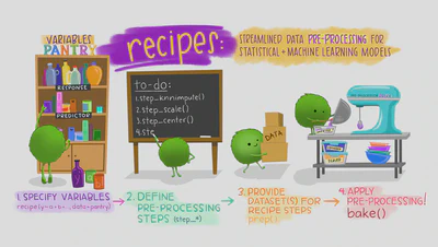
So far we have learned to build linear and logistic regression models, using the parsnip package to specify and train models with different engine. Here we’ll explore another tidymodels package, recipes, which is designed to help you preprocess your data before training your model. Recipes are built as a series of preprocessing steps, such as:
converting qualitative predictors to indicator variables (also known as dummy variables),
transforming data to be on a different scale (e.g., taking the logarithm of a variable),
transforming whole groups of predictors together,
extracting key features from raw variables (e.g., getting the day of the week out of a date variable),
and so on. If you are familiar with R’s formula interface, a lot of this might sound familiar and like what a formula already does. Recipes can be used to do many of the same things, but they have a much wider range of possibilities. This document shows how to use recipes for modeling.
General Social Survey
The General Social Survey is a biannual survey of the American public.
data("gss", package = "rcis")

# select a smaller subset of variables for analysis
gss <- gss %>%
  select(id, wtss, colrac, black, cohort, degree, egalit_scale, owngun, polviews, sex, south)

skimr::skim(gss)
Table: Table 1: Data summary
| Name | gss |
| Number of rows | 1974 |
| Number of columns | 11 |
| _______________________ | |
| Column type frequency: | |
| factor | 7 |
| numeric | 4 |
| ________________________ | |
| Group variables | None |
Variable type: factor
| skim_variable | n_missing | complete_rate | ordered | n_unique | top_counts |
|---|---|---|---|---|---|
| colrac | 702 | 0.64 | FALSE | 2 | NOT: 661, ALL: 611 |
| black | 196 | 0.90 | FALSE | 2 | No: 1477, Yes: 301 |
| degree | 0 | 1.00 | FALSE | 5 | HS: 976, Bac: 354, <HS: 288, Gra: 205 |
| owngun | 669 | 0.66 | FALSE | 3 | NO: 841, YES: 440, REF: 24 |
| polviews | 100 | 0.95 | FALSE | 7 | Mod: 713, Con: 292, Slg: 268, Lib: 244 |
| sex | 0 | 1.00 | FALSE | 2 | Fem: 1088, Mal: 886 |
| south | 0 | 1.00 | FALSE | 2 | Non: 1232, Sou: 742 |
Variable type: numeric
| skim_variable | n_missing | complete_rate | mean | sd | p0 | p25 | p50 | p75 | p100 | hist |
|---|---|---|---|---|---|---|---|---|---|---|
| id | 0 | 1.00 | 987.50 | 569.99 | 1.0 | 494.25 | 987.50 | 1480.75 | 1974.00 | ▇▇▇▇▇ |
| wtss | 0 | 1.00 | 1.00 | 0.62 | 0.4 | 0.82 | 0.82 | 1.24 | 8.74 | ▇▁▁▁▁ |
| cohort | 5 | 1.00 | 1963.81 | 17.69 | 1923.0 | 1951.00 | 1965.00 | 1979.00 | 1994.00 | ▃▆▇▇▇ |
| egalit_scale | 690 | 0.65 | 19.44 | 10.87 | 1.0 | 10.00 | 20.00 | 29.00 | 35.00 | ▆▃▅▅▇ |
rcis::gss contains a selection of variables from the 2012 GSS. We are going to predict attitudes towards racist college professors. Specifically, each respondent was asked “Should a person who believes that Blacks are genetically inferior be allowed to teach in a college or university?” Given the kerfuffle over Richard J. Herrnstein and Charles Murray’s The Bell Curve and the ostracization of Nobel Prize laureate James Watson over his controversial views on race and intelligence, this analysis will provide further insight into the public debate over this issue.
The outcome of interest colrac is a factor variable coded as either "ALLOWED" (respondent believes the person should be allowed to teach) or "NOT ALLOWED" (respondent believes the person should not allowed to teach).
?gss to open a documentation file in R.We can see that about 48% of respondents who answered the question think a person who believes that Blacks are genetically inferior should be allowed to teach in a college or university.
gss %>%
  drop_na(colrac) %>%
  count(colrac) %>%
  mutate(prop = n / sum(n))
## # A tibble: 2 × 3
##   colrac          n  prop
##   <fct>       <int> <dbl>
## 1 ALLOWED       611 0.480
## 2 NOT ALLOWED   661 0.520
Before we start building up our recipe, let’s take a quick look at a few specific variables that will be important for both preprocessing and modeling.
First, notice that the variable colrac is a factor variable; it is important that our outcome variable for training a logistic regression model is a factor.
glimpse(gss)
## Rows: 1,974
## Columns: 11
## $ id           <dbl> 1, 2, 3, 4, 5, 6, 7, 8, 9, 10, 11, 12, 13, 14, 15, 16, 17…
## $ wtss         <dbl> 2.6219629, 3.4959505, 1.7479752, 1.2356944, 0.8739876, 0.…
## $ colrac       <fct> NOT ALLOWED, NOT ALLOWED, NOT ALLOWED, NA, NA, NOT ALLOWE…
## $ black        <fct> No, No, NA, No, Yes, No, No, NA, Yes, No, No, Yes, No, Ye…
## $ cohort       <dbl> 1990, 1991, 1970, 1963, 1942, 1962, 1977, 1988, 1984, 198…
## $ degree       <fct> Bachelor deg, HS, HS, HS, Bachelor deg, Bachelor deg, Jun…
## $ egalit_scale <dbl> NA, 22, 14, 1, 20, NA, 34, 35, NA, 33, NA, 35, 30, NA, 1,…
## $ owngun       <fct> NO, NO, NO, NA, NA, NO, NA, NO, NO, NO, NO, NA, NO, NO, N…
## $ polviews     <fct> Moderate, SlghtCons, SlghtCons, SlghtCons, Liberal, Moder…
## $ sex          <fct> Male, Male, Male, Female, Female, Female, Female, Female,…
## $ south        <fct> Nonsouth, Nonsouth, Nonsouth, Nonsouth, Nonsouth, Nonsout…
Second, there are two variables that we don’t want to use as predictors in our model, but that we would like to retain as identification variables that can be used to troubleshoot poorly predicted data points. These are id and wtss, both numeric values.
Third, there is a substantial amount of missingness to many of the variables in the dataset.
vis_miss(x = gss)
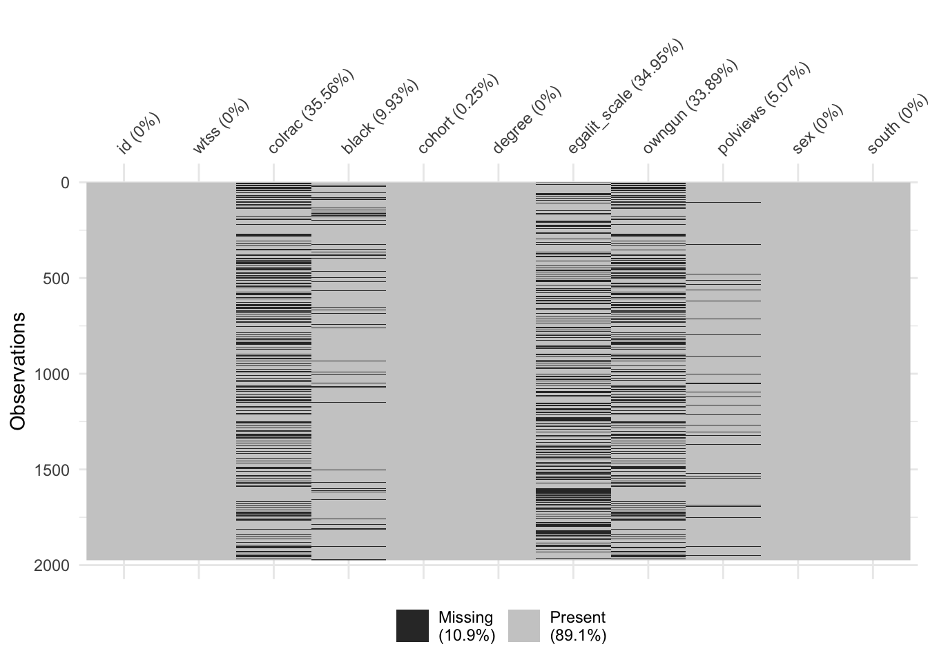
This can make it challenging to estimate a logistic regression model because we can only include observations with complete records (i.e. no missing values on any of the variables). We’ll discuss later in this document specific steps that we can add to our recipe to address this issue before modeling.
Data splitting
To get started, let’s split this single dataset into two: a training set and a testing set. We’ll keep most of the rows in the original dataset (subset chosen randomly) in the training set. The training data will be used to fit the model, and the testing set will be used to measure model performance.
To do this, we can use the rsample package to create an object that contains the information on how to split the data, and then two more rsample functions to create data frames for the training and testing sets:
# Fix the random numbers by setting the seed
# This enables the analysis to be reproducible when random numbers are used
set.seed(123)

# Put 3/4 of the data into the training set
data_split <- initial_split(gss, prop = 3 / 4)

# Create data frames for the two sets:
train_data <- training(data_split)
test_data <- testing(data_split)

nrow(train_data)
## [1] 1480
nrow(test_data)
## [1] 494
Create recipe and roles
To get started, let’s create a recipe for a simple logistic regression model. Before training the model, we can use a recipe to create a few new predictors and conduct some preprocessing required by the model.
Let’s initiate a new recipe:
gss_rec <- recipe(colrac ~ ., data = train_data)
The recipe() function as we used it here has two arguments:
A formula. Any variable on the left-hand side of the tilde (
~) is considered the model outcome (here,colrac). On the right-hand side of the tilde are the predictors. Variables may be listed by name, or you can use the dot (.) to indicate all other variables as predictors.The data. A recipe is associated with the data set used to create the model. This will typically be the training set, so
data = train_datahere. Naming a data set doesn’t actually change the data itself; it is only used to catalog the names of the variables and their types, like factors, integers, dates, etc.
Now we can add roles to this recipe. We can use the update_role() function to let recipes know that id and wtss are variables with a custom role that we called "ID" (a role can have any character value). Whereas our formula included all variables in the training set other than colrac as predictors, this tells the recipe to keep these two variables but not use them as either outcomes or predictors.
gss_rec <- recipe(colrac ~ ., data = train_data) %>%
  update_role(id, wtss, new_role = "ID")
This step of adding roles to a recipe is optional; the purpose of using it here is that those two variables can be retained in the data but not included in the model. This can be convenient when, after the model is fit, we want to investigate some poorly predicted value. These ID columns will be available and can be used to try to understand what went wrong.
To get the current set of variables and roles, use the summary() function:
summary(gss_rec)
## # A tibble: 11 × 4
##    variable     type    role      source
##    <chr>        <chr>   <chr>     <chr>
##  1 id           numeric ID        original
##  2 wtss         numeric ID        original
##  3 black        nominal predictor original
##  4 cohort       numeric predictor original
##  5 degree       nominal predictor original
##  6 egalit_scale numeric predictor original
##  7 owngun       nominal predictor original
##  8 polviews     nominal predictor original
##  9 sex          nominal predictor original
## 10 south        nominal predictor original
## 11 colrac       nominal outcome   original
Create features
Now we can start adding steps onto our recipe using the pipe operator. Perhaps it is reasonable for the birth year of the respondent to have an effect on the likelihood of favoring letting a racist professor teach. A little bit of feature engineering might go a long way to improving our model. How should the birth year be encoded into the model? The cohort column identifies the year of birth for the respondent. Rather than incorporating the variable directly, we can map this onto the respondent’s cultural generation as defined by the Pew Research Center.
Let’s do this by adding steps to our recipe:
gss_rec <- recipe(colrac ~ ., data = train_data) %>%
  update_role(id, wtss, new_role = "ID") %>%
  step_naomit(cohort) %>%
  step_cut(cohort, breaks = c(1945, 1964, 1980))
What do each of these steps do?
- With
step_naomit(), we remove any observations with missing values forcohort(necessary for the following step). - With
step_cut(), we created a factor variable dividing the cohort years into
Next, we’ll turn our attention to the variable types of our predictors. Because we plan to train a logistic regression model, we know that predictors will ultimately need to be numeric, as opposed to factor variables. In other words, there may be a difference in how we store our data (in factors inside a data frame), and how the underlying equations require them (a purely numeric matrix).
For factors like degree and owngun, standard practice is to convert them into dummy or indicator variables to make them numeric. These are binary values for each level of the factor. For example, our owngun variable has values of "YES", "NO", and "REFUSED". The standard dummy variable encoding, shown below, will create two numeric columns of the data that are 1 when the respondent answers "YES" or "NO" and zero otherwise, respectively.
| owngun | owngun_NO | owngun_REFUSED |
|---|---|---|
| NO | 1 | 0 |
| YES | 0 | 0 |
| REFUSED | 0 | 1 |
But, unlike the standard model formula methods in R, a recipe does not automatically create these dummy variables for you; you’ll need to tell your recipe to add this step. This is for two reasons. First, many models do not require numeric predictors, so dummy variables may not always be preferred. Second, recipes can also be used for purposes outside of modeling, where non-dummy versions of the variables may work better. For example, you may want to make a table or a plot with a variable as a single factor. For those reasons, you need to explicitly tell recipes to create dummy variables using step_dummy():
gss_rec <- recipe(colrac ~ ., data = train_data) %>%
  update_role(id, wtss, new_role = "ID") %>%
  step_naomit(cohort) %>%
  step_cut(cohort, breaks = c(1945, 1964, 1980)) %>%
  step_dummy(all_nominal(), -all_outcomes())
Here, we did something different than before: instead of applying a step to an individual variable, we used selectors to apply this recipe step to several variables at once.
The first selector,
all_nominal(), selects all variables that are either factors or characters.The second selector,
-all_outcomes()removes any outcome variables from this recipe step.
With these two selectors together, our recipe step above translates to:
Create dummy variables for all of the factor or character columns unless they are outcomes.
More generally, the recipe selectors mean that you don’t always have to apply steps to individual variables one at a time. Since a recipe knows the variable type and role of each column, they can also be selected (or dropped) using this information.
We need one final step to add to our recipe. Recall that there is substantial missingness throughout the data set. One alternative to excluding all these variables is to impute the missing values by filling them in with plausible alternatives given the overall distribution of values.
recipes supports several different imputation strategies. A simple approach is to fill in the missing values in a column with either the median (for numeric columns) or modal (for categorical columns) values. We can modify our previous recipe to do this.
gss_rec <- recipe(colrac ~ ., data = train_data) %>%
  update_role(id, wtss, new_role = "ID") %>%
  step_impute_median(all_numeric_predictors()) %>%
  step_impute_mode(all_nominal_predictors()) %>%
  step_cut(cohort, breaks = c(1945, 1964, 1980)) %>%
  step_dummy(all_nominal(), -all_outcomes())
Note that I added those steps prior to collapsing the cohort variable. This allows us to avoid removing any observations from the data set prior to modeling the data. I also exclude the outcome and ID variables from the imputation process (all_numeric_predictors()/all_nominal_predictors()) as this imputation approach on the outcome of interest would skew our results.
Now we’ve created a specification of what should be done with the data. How do we use the recipe we made?
Fit a model with a recipe
Let’s use logistic regression to model the GSS data. We start by building a model specification using the parsnip package:
lr_mod <- logistic_reg() %>%
  set_engine("glm")
We will want to use our recipe across several steps as we train and test our model. We will:
Process the recipe using the training set: This involves any estimation or calculations based on the training set. For our recipe, the training set will be used to determine which predictors should be converted to dummy variables and which values will be imputed in the training set.
Apply the recipe to the training set: We create the final predictor set on the training set.
Apply the recipe to the test set: We create the final predictor set on the test set. Nothing is recomputed and no information from the test set is used here; the dummy variable and imputation results from the training set are applied to the test set.
To simplify this process, we can use a model workflow, which pairs a model and recipe together. This is a straightforward approach because different recipes are often needed for different models, so when a model and recipe are bundled, it becomes easier to train and test workflows. We’ll use the workflows package from tidymodels to bundle our parsnip model (lr_mod) with our recipe (gss_rec).
gss_wflow <- workflow() %>%
  add_model(lr_mod) %>%
  add_recipe(gss_rec)
gss_wflow
## ══ Workflow ════════════════════════════════════════════════════════════════════
## Preprocessor: Recipe
## Model: logistic_reg()
##
## ── Preprocessor ────────────────────────────────────────────────────────────────
## 4 Recipe Steps
##
## • step_impute_median()
## • step_impute_mode()
## • step_cut()
## • step_dummy()
##
## ── Model ───────────────────────────────────────────────────────────────────────
## Logistic Regression Model Specification (classification)
##
## Computational engine: glm
Now, there is a single function that can be used to prepare the recipe and train the model from the resulting predictors:
gss_fit <- gss_wflow %>%
  fit(data = train_data)
This object has the finalized recipe and fitted model objects inside. You may want to extract the model or recipe objects from the workflow. To do this, you can use the helper functions extract_fit_parsnip() and extract_recipe(). For example, here we pull the fitted model object then use the broom::tidy() function to get a tidy tibble of model coefficients:
gss_fit %>%
  extract_fit_parsnip() %>%
  tidy()
## # A tibble: 20 × 5
##    term                         estimate std.error statistic p.value
##    <chr>                           <dbl>     <dbl>     <dbl>   <dbl>
##  1 (Intercept)                 -0.0438     0.477     -0.0919 0.927
##  2 egalit_scale                -0.000179   0.00933   -0.0192 0.985
##  3 black_Yes                   -0.0687     0.196     -0.350  0.727
##  4 cohort_X.1.94e.03.1.96e.03. -0.282      0.212     -1.33   0.182
##  5 cohort_X.1.96e.03.1.98e.03. -0.404      0.215     -1.88   0.0603
##  6 cohort_X.1.98e.03.1.99e.03. -0.142      0.229     -0.620  0.535
##  7 degree_HS                    0.0711     0.211      0.338  0.736
##  8 degree_Junior.Coll           0.0391     0.303      0.129  0.897
##  9 degree_Bachelor.deg         -0.294      0.247     -1.19   0.234
## 10 degree_Graduate.deg         -0.372      0.290     -1.28   0.199
## 11 owngun_NO                    0.476      0.150      3.17   0.00154
## 12 owngun_REFUSED               0.907      0.576      1.57   0.115
## 13 polviews_Liberal            -0.120      0.370     -0.324  0.746
## 14 polviews_SlghtLib           -0.732      0.376     -1.95   0.0517
## 15 polviews_Moderate            0.130      0.336      0.387  0.699
## 16 polviews_SlghtCons           0.311      0.370      0.840  0.401
## 17 polviews_Conserv             0.229      0.373      0.614  0.540
## 18 polviews_ExtrmCons          -0.997      0.525     -1.90   0.0574
## 19 sex_Female                   0.156      0.137      1.14   0.254
## 20 south_South                  0.106      0.146      0.726  0.468
Use a trained workflow to predict
Our goal was to predict whether a respondent thinks it is acceptable for a professor with racist views to teach a college class. We have just:
Built the model (
lr_mod),Created a preprocessing recipe (
gss_rec),Bundled the model and recipe (
gss_wflow), andTrained our workflow using a single call to
fit().
The next step is to use the trained workflow (gss_fit) to predict with the unseen test data, which we will do with a single call to predict(). The predict() method applies the recipe to the new data, then passes them to the fitted model.
predict(object = gss_fit, new_data = test_data)
## # A tibble: 494 × 1
##    .pred_class
##    <fct>
##  1 NOT ALLOWED
##  2 NOT ALLOWED
##  3 ALLOWED
##  4 ALLOWED
##  5 ALLOWED
##  6 NOT ALLOWED
##  7 ALLOWED
##  8 ALLOWED
##  9 NOT ALLOWED
## 10 NOT ALLOWED
## # … with 484 more rows
## # ℹ Use `print(n = ...)` to see more rows
Because our outcome variable here is a factor, the output from predict() returns the predicted class: ALLOWED versus NOT ALLOWED. But, let’s say we want the predicted class probabilities for each respondent instead. To return those, we can specify type = "prob" when we use predict(). We’ll also bind the output with some variables from the test data and save them together:
gss_pred <- predict(gss_fit, test_data, type = "prob") %>%
  bind_cols(test_data %>%
    select(colrac))

# The data look like:
gss_pred
## # A tibble: 494 × 3
##   .pred_ALLOWED `.pred_NOT ALLOWED` colrac
##           <dbl>               <dbl> <fct>
## 1         0.399               0.601 NOT ALLOWED
## 2         0.414               0.586 <NA>
## 3         0.700               0.300 <NA>
## 4         0.602               0.398 ALLOWED
## 5         0.726               0.274 NOT ALLOWED
## # … with 489 more rows
## # ℹ Use `print(n = ...)` to see more rows
Now that we have a tibble with our predicted class probabilities, how will we evaluate the performance of our workflow? We can see from these first few rows that our model predicted four of these five respondents correctly because the values of .pred_ALLOWED are p > .50. But we also know that we have 494 rows total to predict. We would like to calculate a metric that tells how well our model predicted respondents’ attitudes, compared to the true status of our outcome variable, colrac.
Let’s use the area under the ROC curve as our metric, computed using roc_curve() and roc_auc() from the yardstick package.
To generate a ROC curve, we need the predicted class probabilities for ALLOWED and NOT ALLOWED, which we just calculated in the code chunk above. We can create the ROC curve with these values, using roc_curve() and then piping to the autoplot() method:
gss_pred %>%
  roc_curve(truth = colrac, .pred_ALLOWED) %>%
  autoplot()
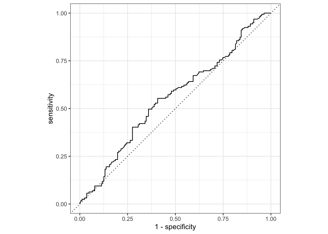
Similarly, roc_auc() estimates the area under the curve:
gss_pred %>%
  roc_auc(truth = colrac, .pred_ALLOWED)
## # A tibble: 1 × 3
##   .metric .estimator .estimate
##   <chr>   <chr>          <dbl>
## 1 roc_auc binary         0.554
Not too bad! With additional variables, further preprocessing, or an alternative modeling strategy, we could improve this model even further.
Acknowledgments
- Example drawn from Get Started - Preprocess your data with
recipesand licensed under CC BY-SA 4.0. - Artwork by @allison_horst
Session Info
sessioninfo::session_info()
## ─ Session info ───────────────────────────────────────────────────────────────
##  setting  value
##  version  R version 4.2.1 (2022-06-23)
##  os       macOS Monterey 12.3
##  system   aarch64, darwin20
##  ui       X11
##  language (EN)
##  collate  en_US.UTF-8
##  ctype    en_US.UTF-8
##  tz       America/New_York
##  date     2022-08-22
##  pandoc   2.18 @ /Applications/RStudio.app/Contents/MacOS/quarto/bin/tools/ (via rmarkdown)
##
## ─ Packages ───────────────────────────────────────────────────────────────────
##  package       * version    date (UTC) lib source
##  assertthat      0.2.1      2019-03-21 [2] CRAN (R 4.2.0)
##  backports       1.4.1      2021-12-13 [2] CRAN (R 4.2.0)
##  base64enc       0.1-3      2015-07-28 [2] CRAN (R 4.2.0)
##  blogdown        1.10       2022-05-10 [2] CRAN (R 4.2.0)
##  bookdown        0.27       2022-06-14 [2] CRAN (R 4.2.0)
##  broom         * 1.0.0      2022-07-01 [2] CRAN (R 4.2.0)
##  bslib           0.4.0      2022-07-16 [2] CRAN (R 4.2.0)
##  cachem          1.0.6      2021-08-19 [2] CRAN (R 4.2.0)
##  cellranger      1.1.0      2016-07-27 [2] CRAN (R 4.2.0)
##  class           7.3-20     2022-01-16 [2] CRAN (R 4.2.1)
##  cli             3.3.0      2022-04-25 [2] CRAN (R 4.2.0)
##  codetools       0.2-18     2020-11-04 [2] CRAN (R 4.2.1)
##  colorspace      2.0-3      2022-02-21 [2] CRAN (R 4.2.0)
##  crayon          1.5.1      2022-03-26 [2] CRAN (R 4.2.0)
##  DBI             1.1.3      2022-06-18 [2] CRAN (R 4.2.0)
##  dbplyr          2.2.1      2022-06-27 [2] CRAN (R 4.2.0)
##  dials         * 1.0.0      2022-06-14 [2] CRAN (R 4.2.0)
##  DiceDesign      1.9        2021-02-13 [2] CRAN (R 4.2.0)
##  digest          0.6.29     2021-12-01 [2] CRAN (R 4.2.0)
##  dplyr         * 1.0.9      2022-04-28 [2] CRAN (R 4.2.0)
##  ellipsis        0.3.2      2021-04-29 [2] CRAN (R 4.2.0)
##  evaluate        0.16       2022-08-09 [1] CRAN (R 4.2.1)
##  fansi           1.0.3      2022-03-24 [2] CRAN (R 4.2.0)
##  fastmap         1.1.0      2021-01-25 [2] CRAN (R 4.2.0)
##  forcats       * 0.5.1      2021-01-27 [2] CRAN (R 4.2.0)
##  foreach         1.5.2      2022-02-02 [2] CRAN (R 4.2.0)
##  fs              1.5.2      2021-12-08 [2] CRAN (R 4.2.0)
##  furrr           0.3.0      2022-05-04 [2] CRAN (R 4.2.0)
##  future          1.27.0     2022-07-22 [2] CRAN (R 4.2.0)
##  future.apply    1.9.0      2022-04-25 [2] CRAN (R 4.2.0)
##  gargle          1.2.0      2021-07-02 [2] CRAN (R 4.2.0)
##  generics        0.1.3      2022-07-05 [2] CRAN (R 4.2.0)
##  ggplot2       * 3.3.6      2022-05-03 [2] CRAN (R 4.2.0)
##  globals         0.16.0     2022-08-05 [2] CRAN (R 4.2.0)
##  glue            1.6.2      2022-02-24 [2] CRAN (R 4.2.0)
##  googledrive     2.0.0      2021-07-08 [2] CRAN (R 4.2.0)
##  googlesheets4   1.0.0      2021-07-21 [2] CRAN (R 4.2.0)
##  gower           1.0.0      2022-02-03 [2] CRAN (R 4.2.0)
##  GPfit           1.0-8      2019-02-08 [2] CRAN (R 4.2.0)
##  gtable          0.3.0      2019-03-25 [2] CRAN (R 4.2.0)
##  hardhat         1.2.0      2022-06-30 [2] CRAN (R 4.2.0)
##  haven           2.5.0      2022-04-15 [2] CRAN (R 4.2.0)
##  here            1.0.1      2020-12-13 [2] CRAN (R 4.2.0)
##  hms             1.1.1      2021-09-26 [2] CRAN (R 4.2.0)
##  htmltools       0.5.3      2022-07-18 [2] CRAN (R 4.2.0)
##  httr            1.4.3      2022-05-04 [2] CRAN (R 4.2.0)
##  infer         * 1.0.2      2022-06-10 [2] CRAN (R 4.2.0)
##  ipred           0.9-13     2022-06-02 [2] CRAN (R 4.2.0)
##  iterators       1.0.14     2022-02-05 [2] CRAN (R 4.2.0)
##  jquerylib       0.1.4      2021-04-26 [2] CRAN (R 4.2.0)
##  jsonlite        1.8.0      2022-02-22 [2] CRAN (R 4.2.0)
##  knitr           1.39       2022-04-26 [2] CRAN (R 4.2.0)
##  lattice         0.20-45    2021-09-22 [2] CRAN (R 4.2.1)
##  lava            1.6.10     2021-09-02 [2] CRAN (R 4.2.0)
##  lhs             1.1.5      2022-03-22 [2] CRAN (R 4.2.0)
##  lifecycle       1.0.1      2021-09-24 [2] CRAN (R 4.2.0)
##  listenv         0.8.0      2019-12-05 [2] CRAN (R 4.2.0)
##  lubridate       1.8.0      2021-10-07 [2] CRAN (R 4.2.0)
##  magrittr        2.0.3      2022-03-30 [2] CRAN (R 4.2.0)
##  MASS            7.3-58.1   2022-08-03 [2] CRAN (R 4.2.0)
##  Matrix          1.4-1      2022-03-23 [2] CRAN (R 4.2.1)
##  modeldata     * 1.0.0      2022-07-01 [2] CRAN (R 4.2.0)
##  modelr          0.1.8      2020-05-19 [2] CRAN (R 4.2.0)
##  munsell         0.5.0      2018-06-12 [2] CRAN (R 4.2.0)
##  naniar        * 0.6.1      2021-05-14 [2] CRAN (R 4.2.0)
##  nnet            7.3-17     2022-01-16 [2] CRAN (R 4.2.1)
##  parallelly      1.32.1     2022-07-21 [2] CRAN (R 4.2.0)
##  parsnip       * 1.0.0      2022-06-16 [2] CRAN (R 4.2.0)
##  pillar          1.8.0      2022-07-18 [2] CRAN (R 4.2.0)
##  pkgconfig       2.0.3      2019-09-22 [2] CRAN (R 4.2.0)
##  prodlim         2019.11.13 2019-11-17 [2] CRAN (R 4.2.0)
##  purrr         * 0.3.4      2020-04-17 [2] CRAN (R 4.2.0)
##  R6              2.5.1      2021-08-19 [2] CRAN (R 4.2.0)
##  rcis          * 0.2.5      2022-08-08 [2] local
##  Rcpp            1.0.9      2022-07-08 [2] CRAN (R 4.2.0)
##  readr         * 2.1.2      2022-01-30 [2] CRAN (R 4.2.0)
##  readxl          1.4.0      2022-03-28 [2] CRAN (R 4.2.0)
##  recipes       * 1.0.1      2022-07-07 [2] CRAN (R 4.2.0)
##  repr            1.1.4      2022-01-04 [2] CRAN (R 4.2.0)
##  reprex          2.0.1.9000 2022-08-10 [1] Github (tidyverse/reprex@6d3ad07)
##  rlang           1.0.4      2022-07-12 [2] CRAN (R 4.2.0)
##  rmarkdown       2.14       2022-04-25 [2] CRAN (R 4.2.0)
##  rpart           4.1.16     2022-01-24 [2] CRAN (R 4.2.1)
##  rprojroot       2.0.3      2022-04-02 [2] CRAN (R 4.2.0)
##  rsample       * 1.1.0      2022-08-08 [2] CRAN (R 4.2.1)
##  rstudioapi      0.13       2020-11-12 [2] CRAN (R 4.2.0)
##  rvest           1.0.2      2021-10-16 [2] CRAN (R 4.2.0)
##  sass            0.4.2      2022-07-16 [2] CRAN (R 4.2.0)
##  scales        * 1.2.0      2022-04-13 [2] CRAN (R 4.2.0)
##  sessioninfo     1.2.2      2021-12-06 [2] CRAN (R 4.2.0)
##  skimr         * 2.1.4      2022-04-15 [2] CRAN (R 4.2.0)
##  stringi         1.7.8      2022-07-11 [2] CRAN (R 4.2.0)
##  stringr       * 1.4.0      2019-02-10 [2] CRAN (R 4.2.0)
##  survival        3.3-1      2022-03-03 [2] CRAN (R 4.2.1)
##  tibble        * 3.1.8      2022-07-22 [2] CRAN (R 4.2.0)
##  tidymodels    * 1.0.0      2022-07-13 [2] CRAN (R 4.2.0)
##  tidyr         * 1.2.0      2022-02-01 [2] CRAN (R 4.2.0)
##  tidyselect      1.1.2      2022-02-21 [2] CRAN (R 4.2.0)
##  tidyverse     * 1.3.2      2022-07-18 [2] CRAN (R 4.2.0)
##  timeDate        4021.104   2022-07-19 [2] CRAN (R 4.2.0)
##  tune          * 1.0.0      2022-07-07 [2] CRAN (R 4.2.0)
##  tzdb            0.3.0      2022-03-28 [2] CRAN (R 4.2.0)
##  utf8            1.2.2      2021-07-24 [2] CRAN (R 4.2.0)
##  vctrs           0.4.1      2022-04-13 [2] CRAN (R 4.2.0)
##  visdat          0.5.3      2019-02-15 [2] CRAN (R 4.2.0)
##  withr           2.5.0      2022-03-03 [2] CRAN (R 4.2.0)
##  workflows     * 1.0.0      2022-07-05 [2] CRAN (R 4.2.0)
##  workflowsets  * 1.0.0      2022-07-12 [2] CRAN (R 4.2.0)
##  xfun            0.31       2022-05-10 [1] CRAN (R 4.2.0)
##  xml2            1.3.3      2021-11-30 [2] CRAN (R 4.2.0)
##  yaml            2.3.5      2022-02-21 [2] CRAN (R 4.2.0)
##  yardstick     * 1.0.0      2022-06-06 [2] CRAN (R 4.2.0)
##
##  [1] /Users/soltoffbc/Library/R/arm64/4.2/library
##  [2] /Library/Frameworks/R.framework/Versions/4.2-arm64/Resources/library
##
## ──────────────────────────────────────────────────────────────────────────────