Logistic regression
library(tidyverse)
library(tidymodels)
set.seed(123)

theme_set(theme_minimal())
Run the code below in your console to download this exercise as a set of R scripts.
usethis::use_course("cis-ds/statistical-learning")
Classification problems
The sinking of RMS Titanic provided the world with many things:
A fundamental shock to the world as its faith in supposedly indestructible technology was shattered by a chunk of ice
Perhaps the best romantic ballad of all time
A tragic love story
)](https://i.giphy.com/KSeT85Vtym7m.gif)
Titanic (1997)
Why did Jack have to die? Why couldn’t he have made it onto a lifeboat like Cal? We may never know the answer, but we can generalize the question a bit: why did some people survive the sinking of the Titanic while others did not?
In essence, we have a classification problem. The response is a binary variable, indicating whether a specific passenger survived. If we combine this with predictors that describe each passenger, we might be able to estimate a general model of survival.1
Kaggle is an online platform for predictive modeling and analytics. They run regular competitions where they provide the public with a question and data, and anyone can estimate a predictive model to answer the question. They’ve run a popular contest based on a dataset of passengers from the Titanic. The datasets have been conveniently stored in a package called titanic. Let’s load the package and convert the desired data frame to a tibble.
library(titanic)
titanic <- titanic_train %>%
  as_tibble()

titanic %>%
  head() %>%
  knitr::kable()
| PassengerId | Survived | Pclass | Name | Sex | Age | SibSp | Parch | Ticket | Fare | Cabin | Embarked |
|---|---|---|---|---|---|---|---|---|---|---|---|
| 1 | 0 | 3 | Braund, Mr. Owen Harris | male | 22 | 1 | 0 | A/5 21171 | 7.2500 | S | |
| 2 | 1 | 1 | Cumings, Mrs. John Bradley (Florence Briggs Thayer) | female | 38 | 1 | 0 | PC 17599 | 71.2833 | C85 | C |
| 3 | 1 | 3 | Heikkinen, Miss. Laina | female | 26 | 0 | 0 | STON/O2. 3101282 | 7.9250 | S | |
| 4 | 1 | 1 | Futrelle, Mrs. Jacques Heath (Lily May Peel) | female | 35 | 1 | 0 | 113803 | 53.1000 | C123 | S |
| 5 | 0 | 3 | Allen, Mr. William Henry | male | 35 | 0 | 0 | 373450 | 8.0500 | S | |
| 6 | 0 | 3 | Moran, Mr. James | male | NA | 0 | 0 | 330877 | 8.4583 | Q |
The codebook contains the following information on the variables:
VARIABLE DESCRIPTIONS:
Survived        Survival
                (0 = No; 1 = Yes)
Pclass          Passenger Class
                (1 = 1st; 2 = 2nd; 3 = 3rd)
Name            Name
Sex             Sex
Age             Age
SibSp           Number of Siblings/Spouses Aboard
Parch           Number of Parents/Children Aboard
Ticket          Ticket Number
Fare            Passenger Fare
Cabin           Cabin
Embarked        Port of Embarkation
                (C = Cherbourg; Q = Queenstown; S = Southampton)

SPECIAL NOTES:
Pclass is a proxy for socio-economic status (SES)
 1st ~ Upper; 2nd ~ Middle; 3rd ~ Lower

Age is in Years; Fractional if Age less than One (1)
 If the Age is Estimated, it is in the form xx.5

With respect to the family relation variables (i.e. sibsp and parch)
some relations were ignored.  The following are the definitions used
for sibsp and parch.

Sibling:  Brother, Sister, Stepbrother, or Stepsister of Passenger Aboard Titanic
Spouse:   Husband or Wife of Passenger Aboard Titanic (Mistresses and Fiances Ignored)
Parent:   Mother or Father of Passenger Aboard Titanic
Child:    Son, Daughter, Stepson, or Stepdaughter of Passenger Aboard Titanic

Other family relatives excluded from this study include cousins,
nephews/nieces, aunts/uncles, and in-laws.  Some children travelled
only with a nanny, therefore parch=0 for them.  As well, some
travelled with very close friends or neighbors in a village, however,
the definitions do not support such relations.
So if this is our data, Survived is our response variable and the remaining variables are predictors. How can we determine who survives and who dies?
A linear regression approach
Let’s concentrate first on the relationship between age and survival. Using the methods we previously learned, we could estimate a linear regression model:
# estimate model
lin_fit <- linear_reg() %>%
  set_engine("lm") %>%
  fit(Survived ~ Age, data = titanic)

# visualize predicted values
age_vals <- tibble(
  Age = 0:80
)

bind_cols(
  age_vals,
  predict(lin_fit, new_data = age_vals)
) %>%
  ggplot(mapping = aes(x = Age, y = .pred)) +
  geom_point(data = titanic, mapping = aes(x = Age, y = Survived)) +
  geom_line() +
  ylim(0, 1)
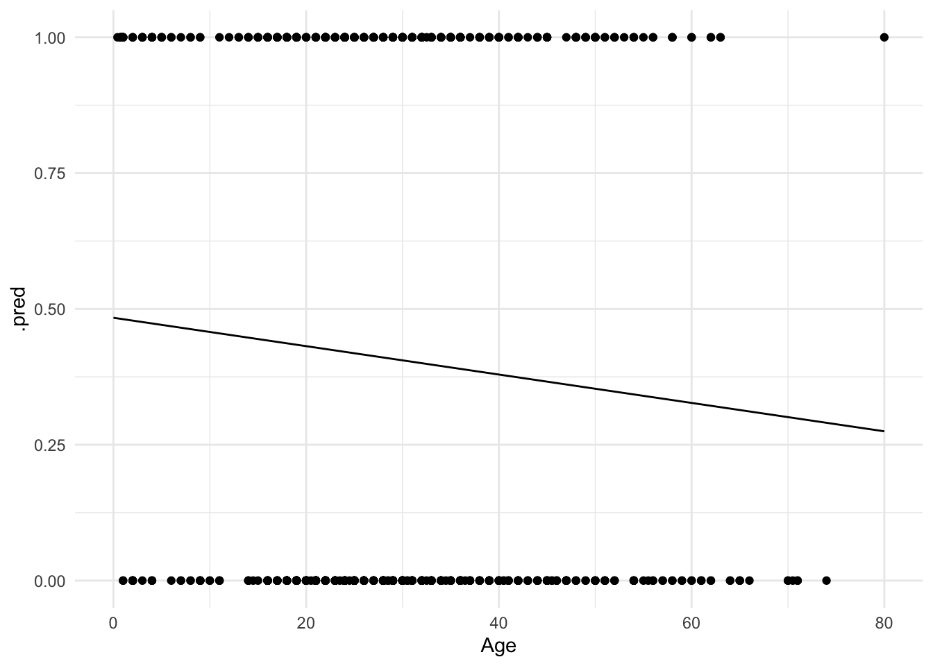
Hmm. Not terrible, but you can immediately notice a couple of things. First, the only possible values for Survival are $0$ and $1$. Yet the linear regression model gives us predicted values such as $.4$ and $.25$. How should we interpret those?
One possibility is that these values are predicted probabilities. That is, the estimated probability a passenger will survive given their age. So someone with a predicted probability of $.4$ has a 40% chance of surviving. Okay, but notice that because the line is linear and continuous, it extends infinitely in both directions of age.
# visualize predicted values
age_vals <- tibble(
  Age = 0:200
)

bind_cols(
  age_vals,
  predict(lin_fit, new_data = age_vals)
) %>%
  ggplot(mapping = aes(x = Age, y = .pred)) +
  geom_point(data = titanic, mapping = aes(x = Age, y = Survived)) +
  geom_line() +
  ylim(NA, 1)
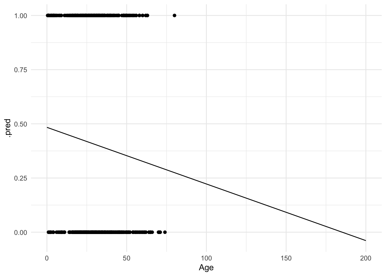
What happens if a 200 year old person is on the Titanic? They would have a $-.1$ probability of surviving. But you cannot have a probability outside of the $[0,1]$ interval! Admittedly this is a trivial example, but in other circumstances this can become a more realistic scenario.
Or what if we didn’t want to predict survival, but instead predict the port from which an individual departed (Cherbourg, Queenstown, or Southampton)? We could try and code this as a numeric response variable:
| Numeric value | Port |
|---|---|
| 1 | Cherbourg |
| 2 | Queenstown |
| 3 | Southampton |
But why not instead code it:
| Numeric value | Port |
|---|---|
| 1 | Queenstown |
| 2 | Cherbourg |
| 3 | Southampton |
Or even:
| Numeric value | Port |
|---|---|
| 1 | Southampton |
| 2 | Cherbourg |
| 3 | Queenstown |
There is no inherent ordering to this variable. Any claimed linear relationship between a predictor and port of embarkation is completely dependent on how we convert the classes to numeric values.
Logistic regression
Rather than modeling the response $Y$ directly, logistic regression instead models the probability that $Y$ belongs to a particular category. In our first Titanic example, the probability of survival can be written as:
$$\Pr(\text{survival} = \text{Yes} | \text{age})$$
The values of $\Pr(\text{survival} = \text{Yes} | \text{age})$ (or simply $\Pr(\text{survival})$) will range between 0 and 1. Given that predicted probability, we could predict anyone with for whom $\Pr(\text{survival}) > .5$ will survive the sinking, and anyone else will die.2
Using tidymodels and the parsnip package, we can estimate this model. Unlike our previous example, we will use logistic_reg() since we are working with a binary outcome. Note that we also need to ensure our outcome variable (Survived) is stored as a factor column so that parsnip recognizes it as a categorical variable.
titanic <- titanic_train %>%
  as_tibble() %>%
  # convert Survived to factor column
  mutate(Survived = factor(
    x = Survived,
    levels = 0:1,
    labels = c("No", "Yes")
  ))
log_mod <- logistic_reg() %>%
  set_engine("glm")

log_fit <- log_mod %>%
  fit(Survived ~ Age, data = titanic)
log_fit
## parsnip model object
##
##
## Call:  stats::glm(formula = Survived ~ Age, family = stats::binomial,
##     data = data)
##
## Coefficients:
## (Intercept)          Age
##    -0.05672     -0.01096
##
## Degrees of Freedom: 713 Total (i.e. Null);  712 Residual
##   (177 observations deleted due to missingness)
## Null Deviance:	    964.5
## Residual Deviance: 960.2 	AIC: 964.2
tidy(log_fit)
## # A tibble: 2 × 5
##   term        estimate std.error statistic p.value
##   <chr>          <dbl>     <dbl>     <dbl>   <dbl>
## 1 (Intercept)  -0.0567   0.174      -0.327  0.744
## 2 Age          -0.0110   0.00533    -2.06   0.0397
Which produces a line that looks like this:
# estimate predicted probabilities
new_ages <- tibble(Age = 0:80)
new_ages_pred <- predict(log_fit, new_data = new_ages, type = "prob")

# visualize results
new_ages %>%
  bind_cols(new_ages_pred) %>%
  ggplot(mapping = aes(x = Age, y = .pred_Yes)) +
  geom_line() +
  ylim(0, 1) +
  ylab("Probability of survival")
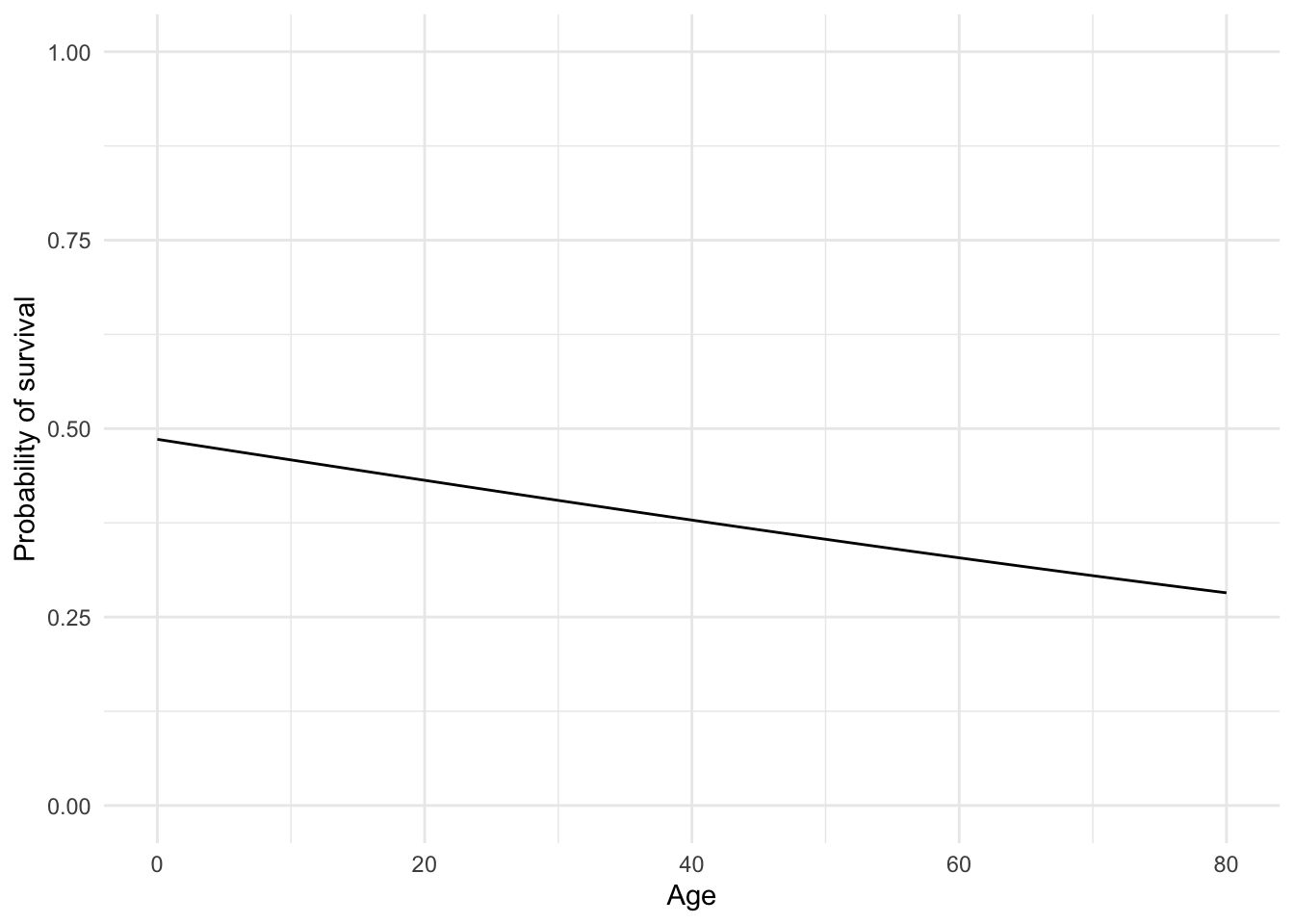
It’s hard to tell, but the line is not perfectly linear. Let’s expand the range of the x-axis to prove this:
# estimate predicted probabilities
new_ages <- tibble(Age = 0:200)
new_ages_pred <- predict(log_fit, new_data = new_ages, type = "prob")

# visualize results
new_ages %>%
  bind_cols(new_ages_pred) %>%
  ggplot(mapping = aes(x = Age, y = .pred_Yes)) +
  geom_line() +
  ylim(0, 1) +
  ylab("Probability of survival")
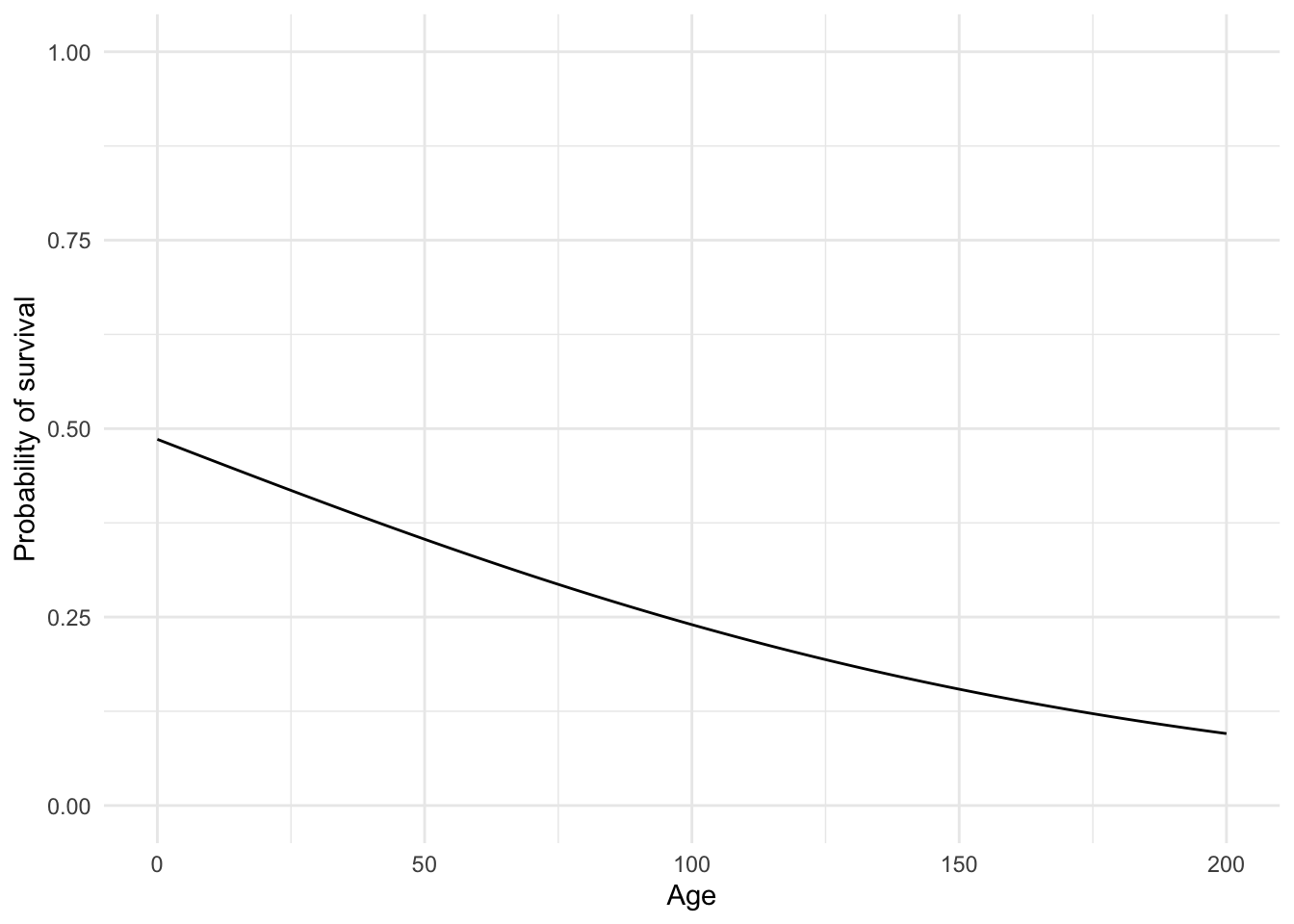
No more predictions that a 200 year old has a $-.1$ probability of surviving!
Multiple predictors
But as the old principle of the sea goes, “women and children first”. What if age isn’t the only factor effecting survival? Fortunately logistic regression handles multiple predictors:
mult_fit <- log_mod %>%
  fit(Survived ~ Age + Sex, data = titanic)
tidy(mult_fit)
## # A tibble: 3 × 5
##   term        estimate std.error statistic  p.value
##   <chr>          <dbl>     <dbl>     <dbl>    <dbl>
## 1 (Intercept)  1.28      0.230       5.55  2.87e- 8
## 2 Age         -0.00543   0.00631    -0.860 3.90e- 1
## 3 Sexmale     -2.47      0.185     -13.3   2.26e-40
The coefficients essentially tell us the relationship between each individual predictor and the response, independent of other predictors. So this model tells us the relationship between age and survival, after controlling for the effects of sex. Likewise, it also tells us the relationship between sex and survival, after controlling for the effects of age.
To get a better visualization of this, let’s again use predict() to generate predicted values for individuals based on their ages and sex:
age_sex_vals <- expand.grid(
  Age = 0:80,
  Sex = c("male", "female")
)

age_sex_pred <- predict(mult_fit, new_data = age_sex_vals, type = "prob")

age_sex_vals %>%
  bind_cols(age_sex_pred) %>%
  ggplot(mapping = aes(
    x = Age,
    y = .pred_Yes,
    color = Sex
  )) +
  geom_line() +
  labs(
    title = "Probability of Surviving the Titanic",
    y = "Predicted Probability of Survival",
    color = "Sex"
  ) +
  scale_color_viridis_d(end = 0.7)
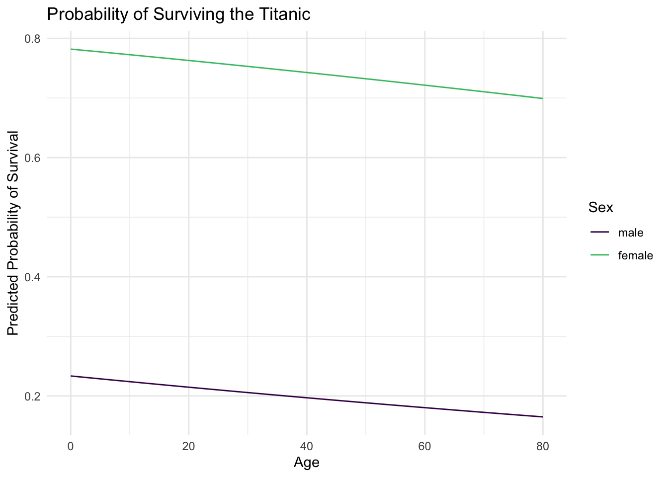
This graph illustrates a key fact about surviving the sinking of the Titanic - age was not really a dominant factor. Instead, one’s sex was much more important. Females survived at much higher rates than males, regardless of age.
Interactive terms
Another assumption of linear and logistic regression is that the relationships between predictors and responses are independent from one another. So for the age and sex example, we assume our function $f$ looks something like:3
$$f = \beta_{0} + \beta_{1}\text{age} + \beta_{2}\text{sex}$$
However once again, that is an assumption. What if the relationship between age and the probability of survival is actually dependent on whether or not the individual is a female? This possibility would take the functional form:
$$f = \beta_{0} + \beta_{1}\text{age} + \beta_{2}\text{sex} + \beta_{3}(\text{age} \times \text{sex})$$
This is considered an interaction between age and sex. To estimate this in R, we simply specify Age * Sex in our formula in fit():4
int_fit <- log_mod %>%
  fit(Survived ~ Age * Sex, data = titanic)
tidy(int_fit)
## # A tibble: 4 × 5
##   term        estimate std.error statistic p.value
##   <chr>          <dbl>     <dbl>     <dbl>   <dbl>
## 1 (Intercept)   0.594     0.310       1.91 0.0557
## 2 Age           0.0197    0.0106      1.86 0.0624
## 3 Sexmale      -1.32      0.408      -3.23 0.00125
## 4 Age:Sexmale  -0.0411    0.0136     -3.03 0.00241
As before, let’s estimate predicted probabilities and plot the interactive effects of age and sex.
int_pred <- predict(int_fit, new_data = age_sex_vals, type = "prob")

age_sex_vals %>%
  bind_cols(int_pred) %>%
  ggplot(mapping = aes(
    x = Age,
    y = .pred_Yes,
    color = Sex
  )) +
  geom_line() +
  labs(
    title = "Probability of Surviving the Titanic",
    y = "Predicted Probability of Survival",
    color = "Sex"
  ) +
  scale_color_viridis_d(end = 0.7)
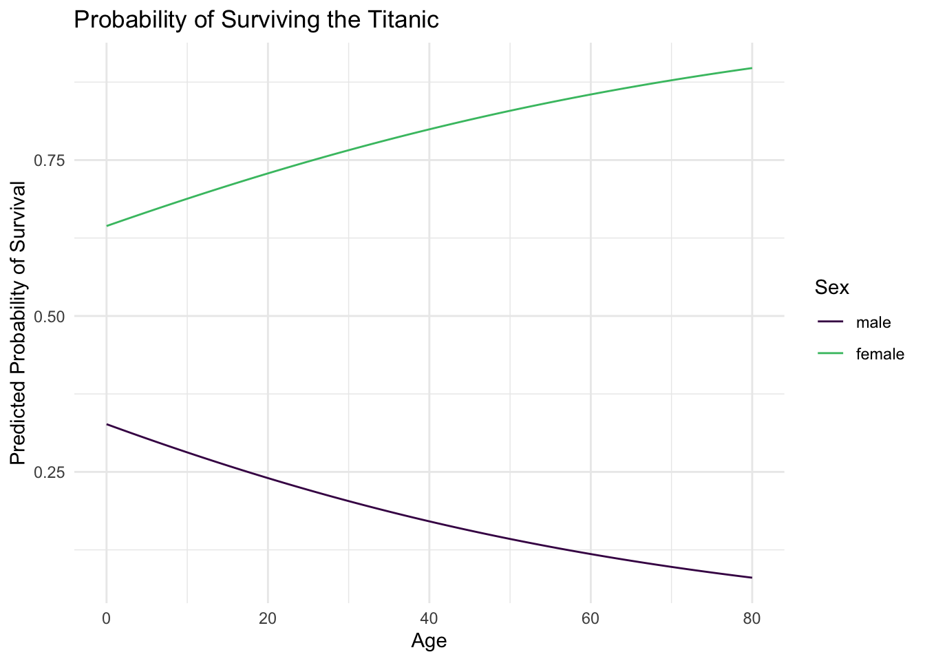
And now our minds are blown once again! For women, as age increases the probability of survival also increases. However for men, we see the opposite relationship: as age increases the probability of survival decreases. Again, the basic principle of saving women and children first can be seen empirically in the estimated probability of survival. Male children are treated similarly to female children, and their survival is prioritized. Even still, the odds of survival are always worse for men than women, but the regression function clearly shows a difference from our previous results.
You may think then that it makes sense to throw in interaction terms willy-nilly to all your regression models since we never know for sure if the relationship is strictly linear and independent. You could do that, but once you start adding more predictors (3, 4, 5, etc.) that will get very difficult to keep track of (five-way interactions are extremely difficult to interpret - even three-way get to be problematic). The best advice is to use theory and your domain knowledge as your guide. Do you have a reason to believe the relationship should be interactive? If so, test for it. If not, don’t.
Session Info
sessioninfo::session_info()
## ─ Session info ───────────────────────────────────────────────────────────────
##  setting  value
##  version  R version 4.2.1 (2022-06-23)
##  os       macOS Monterey 12.3
##  system   aarch64, darwin20
##  ui       X11
##  language (EN)
##  collate  en_US.UTF-8
##  ctype    en_US.UTF-8
##  tz       America/New_York
##  date     2022-08-22
##  pandoc   2.18 @ /Applications/RStudio.app/Contents/MacOS/quarto/bin/tools/ (via rmarkdown)
##
## ─ Packages ───────────────────────────────────────────────────────────────────
##  package       * version    date (UTC) lib source
##  assertthat      0.2.1      2019-03-21 [2] CRAN (R 4.2.0)
##  backports       1.4.1      2021-12-13 [2] CRAN (R 4.2.0)
##  blogdown        1.10       2022-05-10 [2] CRAN (R 4.2.0)
##  bookdown        0.27       2022-06-14 [2] CRAN (R 4.2.0)
##  broom         * 1.0.0      2022-07-01 [2] CRAN (R 4.2.0)
##  bslib           0.4.0      2022-07-16 [2] CRAN (R 4.2.0)
##  cachem          1.0.6      2021-08-19 [2] CRAN (R 4.2.0)
##  cellranger      1.1.0      2016-07-27 [2] CRAN (R 4.2.0)
##  class           7.3-20     2022-01-16 [2] CRAN (R 4.2.1)
##  cli             3.3.0      2022-04-25 [2] CRAN (R 4.2.0)
##  codetools       0.2-18     2020-11-04 [2] CRAN (R 4.2.1)
##  colorspace      2.0-3      2022-02-21 [2] CRAN (R 4.2.0)
##  crayon          1.5.1      2022-03-26 [2] CRAN (R 4.2.0)
##  DBI             1.1.3      2022-06-18 [2] CRAN (R 4.2.0)
##  dbplyr          2.2.1      2022-06-27 [2] CRAN (R 4.2.0)
##  dials         * 1.0.0      2022-06-14 [2] CRAN (R 4.2.0)
##  DiceDesign      1.9        2021-02-13 [2] CRAN (R 4.2.0)
##  digest          0.6.29     2021-12-01 [2] CRAN (R 4.2.0)
##  dplyr         * 1.0.9      2022-04-28 [2] CRAN (R 4.2.0)
##  ellipsis        0.3.2      2021-04-29 [2] CRAN (R 4.2.0)
##  evaluate        0.16       2022-08-09 [1] CRAN (R 4.2.1)
##  fansi           1.0.3      2022-03-24 [2] CRAN (R 4.2.0)
##  fastmap         1.1.0      2021-01-25 [2] CRAN (R 4.2.0)
##  forcats       * 0.5.1      2021-01-27 [2] CRAN (R 4.2.0)
##  foreach         1.5.2      2022-02-02 [2] CRAN (R 4.2.0)
##  fs              1.5.2      2021-12-08 [2] CRAN (R 4.2.0)
##  furrr           0.3.0      2022-05-04 [2] CRAN (R 4.2.0)
##  future          1.27.0     2022-07-22 [2] CRAN (R 4.2.0)
##  future.apply    1.9.0      2022-04-25 [2] CRAN (R 4.2.0)
##  gargle          1.2.0      2021-07-02 [2] CRAN (R 4.2.0)
##  generics        0.1.3      2022-07-05 [2] CRAN (R 4.2.0)
##  ggplot2       * 3.3.6      2022-05-03 [2] CRAN (R 4.2.0)
##  globals         0.16.0     2022-08-05 [2] CRAN (R 4.2.0)
##  glue            1.6.2      2022-02-24 [2] CRAN (R 4.2.0)
##  googledrive     2.0.0      2021-07-08 [2] CRAN (R 4.2.0)
##  googlesheets4   1.0.0      2021-07-21 [2] CRAN (R 4.2.0)
##  gower           1.0.0      2022-02-03 [2] CRAN (R 4.2.0)
##  GPfit           1.0-8      2019-02-08 [2] CRAN (R 4.2.0)
##  gtable          0.3.0      2019-03-25 [2] CRAN (R 4.2.0)
##  hardhat         1.2.0      2022-06-30 [2] CRAN (R 4.2.0)
##  haven           2.5.0      2022-04-15 [2] CRAN (R 4.2.0)
##  here            1.0.1      2020-12-13 [2] CRAN (R 4.2.0)
##  hms             1.1.1      2021-09-26 [2] CRAN (R 4.2.0)
##  htmltools       0.5.3      2022-07-18 [2] CRAN (R 4.2.0)
##  httr            1.4.3      2022-05-04 [2] CRAN (R 4.2.0)
##  infer         * 1.0.2      2022-06-10 [2] CRAN (R 4.2.0)
##  ipred           0.9-13     2022-06-02 [2] CRAN (R 4.2.0)
##  iterators       1.0.14     2022-02-05 [2] CRAN (R 4.2.0)
##  jquerylib       0.1.4      2021-04-26 [2] CRAN (R 4.2.0)
##  jsonlite        1.8.0      2022-02-22 [2] CRAN (R 4.2.0)
##  knitr           1.39       2022-04-26 [2] CRAN (R 4.2.0)
##  lattice         0.20-45    2021-09-22 [2] CRAN (R 4.2.1)
##  lava            1.6.10     2021-09-02 [2] CRAN (R 4.2.0)
##  lhs             1.1.5      2022-03-22 [2] CRAN (R 4.2.0)
##  lifecycle       1.0.1      2021-09-24 [2] CRAN (R 4.2.0)
##  listenv         0.8.0      2019-12-05 [2] CRAN (R 4.2.0)
##  lubridate       1.8.0      2021-10-07 [2] CRAN (R 4.2.0)
##  magrittr        2.0.3      2022-03-30 [2] CRAN (R 4.2.0)
##  MASS            7.3-58.1   2022-08-03 [2] CRAN (R 4.2.0)
##  Matrix          1.4-1      2022-03-23 [2] CRAN (R 4.2.1)
##  modeldata     * 1.0.0      2022-07-01 [2] CRAN (R 4.2.0)
##  modelr          0.1.8      2020-05-19 [2] CRAN (R 4.2.0)
##  munsell         0.5.0      2018-06-12 [2] CRAN (R 4.2.0)
##  nnet            7.3-17     2022-01-16 [2] CRAN (R 4.2.1)
##  parallelly      1.32.1     2022-07-21 [2] CRAN (R 4.2.0)
##  parsnip       * 1.0.0      2022-06-16 [2] CRAN (R 4.2.0)
##  pillar          1.8.0      2022-07-18 [2] CRAN (R 4.2.0)
##  pkgconfig       2.0.3      2019-09-22 [2] CRAN (R 4.2.0)
##  prodlim         2019.11.13 2019-11-17 [2] CRAN (R 4.2.0)
##  purrr         * 0.3.4      2020-04-17 [2] CRAN (R 4.2.0)
##  R6              2.5.1      2021-08-19 [2] CRAN (R 4.2.0)
##  Rcpp            1.0.9      2022-07-08 [2] CRAN (R 4.2.0)
##  readr         * 2.1.2      2022-01-30 [2] CRAN (R 4.2.0)
##  readxl          1.4.0      2022-03-28 [2] CRAN (R 4.2.0)
##  recipes       * 1.0.1      2022-07-07 [2] CRAN (R 4.2.0)
##  reprex          2.0.1.9000 2022-08-10 [1] Github (tidyverse/reprex@6d3ad07)
##  rlang           1.0.4      2022-07-12 [2] CRAN (R 4.2.0)
##  rmarkdown       2.14       2022-04-25 [2] CRAN (R 4.2.0)
##  rpart           4.1.16     2022-01-24 [2] CRAN (R 4.2.1)
##  rprojroot       2.0.3      2022-04-02 [2] CRAN (R 4.2.0)
##  rsample       * 1.1.0      2022-08-08 [2] CRAN (R 4.2.1)
##  rstudioapi      0.13       2020-11-12 [2] CRAN (R 4.2.0)
##  rvest           1.0.2      2021-10-16 [2] CRAN (R 4.2.0)
##  sass            0.4.2      2022-07-16 [2] CRAN (R 4.2.0)
##  scales        * 1.2.0      2022-04-13 [2] CRAN (R 4.2.0)
##  sessioninfo     1.2.2      2021-12-06 [2] CRAN (R 4.2.0)
##  stringi         1.7.8      2022-07-11 [2] CRAN (R 4.2.0)
##  stringr       * 1.4.0      2019-02-10 [2] CRAN (R 4.2.0)
##  survival        3.3-1      2022-03-03 [2] CRAN (R 4.2.1)
##  tibble        * 3.1.8      2022-07-22 [2] CRAN (R 4.2.0)
##  tidymodels    * 1.0.0      2022-07-13 [2] CRAN (R 4.2.0)
##  tidyr         * 1.2.0      2022-02-01 [2] CRAN (R 4.2.0)
##  tidyselect      1.1.2      2022-02-21 [2] CRAN (R 4.2.0)
##  tidyverse     * 1.3.2      2022-07-18 [2] CRAN (R 4.2.0)
##  timeDate        4021.104   2022-07-19 [2] CRAN (R 4.2.0)
##  tune          * 1.0.0      2022-07-07 [2] CRAN (R 4.2.0)
##  tzdb            0.3.0      2022-03-28 [2] CRAN (R 4.2.0)
##  utf8            1.2.2      2021-07-24 [2] CRAN (R 4.2.0)
##  vctrs           0.4.1      2022-04-13 [2] CRAN (R 4.2.0)
##  withr           2.5.0      2022-03-03 [2] CRAN (R 4.2.0)
##  workflows     * 1.0.0      2022-07-05 [2] CRAN (R 4.2.0)
##  workflowsets  * 1.0.0      2022-07-12 [2] CRAN (R 4.2.0)
##  xfun            0.31       2022-05-10 [1] CRAN (R 4.2.0)
##  xml2            1.3.3      2021-11-30 [2] CRAN (R 4.2.0)
##  yaml            2.3.5      2022-02-21 [2] CRAN (R 4.2.0)
##  yardstick     * 1.0.0      2022-06-06 [2] CRAN (R 4.2.0)
##
##  [1] /Users/soltoffbc/Library/R/arm64/4.2/library
##  [2] /Library/Frameworks/R.framework/Versions/4.2-arm64/Resources/library
##
## ──────────────────────────────────────────────────────────────────────────────
General at least as applied to the Titanic. I’d like to think technology has advanced some since the early 20th century that the same patterns do not apply today. Not that sinking ships have gone away. ↩︎
The threshold can be adjusted depending on how conservative or risky of a prediction you wish to make. ↩︎
In mathematical truth, it looks more like $\Pr(\text{survival} = \text{Yes} | \text{age}, \text{sex}) = \frac{1}{1 + e^{-(\beta_{0} + \beta_{1}\text{age} + \beta_{2}\text{sex})}}$. ↩︎
R automatically includes constituent terms, so this turns into
Age + Sex + Age * Sex. Generally you always want to include constituent terms in a regression model with an interaction. ↩︎