Introduction to the course
Who am I?
Me (Dr. Benjamin Soltoff)
I am Lecturer in Information Science in the information science department. Previously I was Assistant Senior Instructional Professor in Computational Social Science and Associate Director of the Masters in Computational Social Science program. I earned my PhD in political science from Penn State University. My research interests focus on judicial politics, state courts, and agenda-setting. Methodologically I am interested in statistical learning and text analysis.
I was first drawn to programming in grad school, starting out in Stata and eventually making the transition to R and Python. I learned these programming languages out of necessity - I needed to process, analyze, and code tens of thousands of judicial opinions and extract key information into a tabular format. I am not a computer scientist. I am a social scientist who uses programming and computational tools to answer my research questions.
Teaching assistants
- Catherine Yu
- Andrew Liu
Course objectives
The goal of this course is to teach you basic computational skills and provide you with the means to learn what you need to know for your own research. I start from the perspective that you want to analyze data, and programming is a means to that end. You will not become an expert programmer - that is a given. But you will learn the basic skills and techniques necessary to conduct data science, and gain the confidence necessary to learn new techniques as you encounter them in your research.
We will cover many different topics in this course, including:
- Elementary programming techniques (e.g. loops, conditional statements, functions)
- Writing reusable, interpretable code
- Problem-solving - debugging programs for errors
- Obtaining, importing, and munging data from a variety of sources
- Performing statistical analysis
- Visualizing information
- Creating interactive reports
- Generating reproducible research
How we will do this
This is a hands-on class. You will learn by writing programs and analysis. Don’t fear the word “program”. A program can be as simple as:
print("Hello world")
## [1] "Hello world"
One line of code, and it performs a very specific task (print the phrase “Hello world” to the screen).
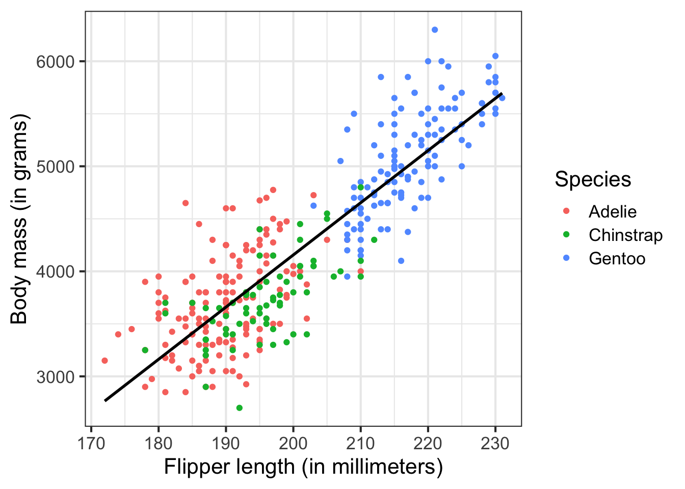
More typically, your programs will perform statistical and graphical analysis on data of a variety of forms. For example, here I analyze a dataset of adult foraging penguins to assess the relationship between flipper length and body mass:
# load packages
library(tidyverse)
## ── Attaching packages ─────────────────────────────────────── tidyverse 1.3.2 ──
## ✔ ggplot2 3.3.6     ✔ purrr   0.3.4
## ✔ tibble  3.1.8     ✔ dplyr   1.0.9
## ✔ tidyr   1.2.0     ✔ stringr 1.4.0
## ✔ readr   2.1.2     ✔ forcats 0.5.1
## ── Conflicts ────────────────────────────────────────── tidyverse_conflicts() ──
## ✖ dplyr::filter() masks stats::filter()
## ✖ dplyr::lag()    masks stats::lag()
library(palmerpenguins)
library(broom)

# estimate and print the linear model
lm(body_mass_g ~ flipper_length_mm, data = penguins) %>%
  tidy() %>%
  mutate(term = c("Intercept", "Flipper length (millimeters)")) %>%
  knitr::kable(
    digits = 2,
    col.names = c(
      "Variable", "Estimate", "Standard Error",
      "T-statistic", "P-Value"
    )
  )
| Variable | Estimate | Standard Error | T-statistic | P-Value |
|---|---|---|---|---|
| Intercept | -5780.83 | 305.81 | -18.90 | 0 |
| Flipper length (millimeters) | 49.69 | 1.52 | 32.72 | 0 |
# visualize the relationship
ggplot(data = penguins, aes(x = flipper_length_mm, y = body_mass_g)) +
  geom_point(mapping = aes(color = species)) +
  geom_smooth(method = "lm", se = FALSE, color = "black", alpha = .25) +
  labs(
    x = "Flipper length (in millimeters)",
    y = "Body mass (in grams)",
    color = "Species"
  ) +
  theme_bw(base_size = 16)
## `geom_smooth()` using formula 'y ~ x'
But we will start small to build our way up to there.
Class sessions will include a combination of lecture and live-coding. You need to bring a laptop to class to follow along, but all class materials (including slides and notes) will be made available before/after class for your review. The emphasis of the class is on application and learning how to implement different computational techniques. However we will sometimes read and discuss examples of interesting and relevant scholarly research that demonstrates the capabilities and range of computational social science.
Complete the readings
Each class will have assigned readings. You need to complete these before coming to class. I will assume you have done so and have at least a basic understanding of the material. My general structure for the class is to spend the first 15-30 minutes lecturing, then the remaining time practicing skills via live-coding and in-class exercises. If you do not come to class prepared, then there is no point in coming to class.
15 minute rule
You will fail in this class. You will stumble, you will get lost, confused, not understand how to perform a task, not understand why your code is generating an error. But as Alfred so helpfully points out to Bruce Wayne, do not fall to pieces when you fail. Instead, learn to pick yourself up, recover, and learn from the experience. Consider this a lesson not only for this class, but graduate school in general.
We will follow the 15 minute rule in this class.1 If you encounter a problem in your assignments, spend 15 minutes troubleshooting the problem on your own. Make use of Google and StackOverflow to resolve the error. However, if after 15 minutes you still cannot solve the problem, ask for help. We will use GitHub to ask and answer class-related questions.
Plagiarism
I am trying to balance two competing perspectives:
- Collaboration is good - researchers usually collaborate with one another on projects. Developers work in teams to write programs. Why reinvent the wheel when it has already been done?
- Collaboration is cheating - this is academia. You are expected to complete your own work. If you copy from someone else, how do I know you actually learned the material?
The point is that collaboration in this class is good - to a point. You are always, unless otherwise noted, expected to write and submit your own work. You should not blindly copy from your peers. You should not copy large chunks of code from the internet. That said, using the internet to debug programs is fine. Asking a classmate to help you debug your program is fine (the key phrase is help you, not do it for you).
The bottom line - if you don’t understand what the program is doing and are not prepared to explain it in detail, you should not submit it.
Evaluations
You will complete a series of programming assignments throughout the semester linked to lecture materials. These assignments will generally be due the following week prior to Monday’s class. Assignments will initially come with starter code, or an initial version of the program where you need to fill in the blanks to make it work. As the semester moves on and your skills become more developed, I will provide less help upfront.
Each assignment will be evaluated by myself or a TA, as well as by two peers. Peer review is a crucial element to this course, in that by eating each other’s dog food you will learn to read, debug, and reproduce code and analysis. And while I and the TAs are competent users in R, your classmates are not - so make sure your code is well-documented so that others with basic knowledge of programming and R can follow along and reuse your code. Be sure to read the instructions for peer review so you know how to provide useful feedback.
The data workflow
 by Garrett Grolemund and Hadley Wickham.](/media/data-science_huf85a0f02017eed09135d1a4755c44d35_13579_eb5214fad9f651689846929f7be18a02.webp)
Computationally driven research follows a specific workflow. This is the ideal - in this course, I want to illustrate and explain to you why each stage is important and how to do it.
Import
First you need to get your data into whatever software package you will use to analyze it. Most of us are familiar with data stored in flat files (e.g. spreadsheets). However a lot of interesting data cannot be obtained in a single specific and simple format. Information you need could be stored in a database, or a web API, or even (gasp!) printed books. You need to know how to convert/extract information into your software package of choice.
Tidy
Tidying your data means to store it in a standardized form that enables the use of a standard library of functions to analyze the data. When your data is tidy, each column is a variable, and each row is an observation. By storing data in a consistent structure, you can focus your efforts on questions about the data and not constantly wrangling the data into different forms. Contrary to what you might expect, much of a researcher’s time is spent wrangling and cleaning data into a tidy format for analysis. While not glamorous, tidying is an important stage.
Transform
Transforming data can take on different tasks. Typically these include subsetting the data to focus on one specific set of observations, creating new variables that are functions of existing variables, or calculating summary statistics for the data.
Visualize
Humans love to visualize information, as it reduces the complexity of the data into an easily interpretable format. There are many different ways to visualize data - knowing how to create specific graphs is important, but even more so is the ability to determine what visualizations are appropriate given the variables you wish to analyze.
Model
Models complement visualizations. While visualizations are intuitive, they do not scale well to complex relationships. Visualizing two (or even three) variables is a straightforward exercise, but once you are dealing with four or more variables visualizations become pointless. Models are fundamentally mathemetical, so they scale well to many variables. However all models make assumptions about the form of relationships, so if you choose an inappropriate functional form the model will not tell you that you are wrong.
Communicate
All of the above work will be for naught if you fail to communicate your project to a larger audience. You need to not only understand your data, but also communicate your results to others so that the community can learn from your knowledge.
Programming
Programming is the tool that encompasses all of the previous stages. You can use programming in all facets of your project. You do not need to be an expert programmer to be a computational social scientist, but learning to program will make your life much easier.
Basic principles of programming
A program is a series of instructions that specifies how to perform a computation.2
Major components to programs are:
- Input - what is being manipulated/utilized. Typically these are data files from your hard drive or the internet.
- Output - display data or analysis on the computer, include in a paper/report, publish on the internet, etc.
- Math - basic or complex mathematical and statistical operations. This could be as simple as addition or subtraction, or more complicated like estimating a linear regression or statistical learning model.
- Conditional execution - check for certain conditions and only perform operations when conditions are met.
- Repetition - perform some action repeatedly, usually with some variation.
Virtually all programs are built using these fundamental components. Obviously the more components you implement, the more complex the program will become. The skill is in breaking up a problem into smaller parts until each part is simple enough to be computed using these basic instructions.
GUI software
A graphical user interface (GUI) is a visual way of interacting with a computer using elements such as a mouse, icons, and menus.
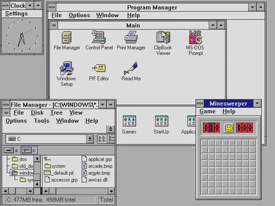
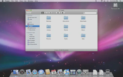

GUI software runs using all the basic programming elements, but the end user is not aware of any of this. Instructions in GUI software are implicit to the user, whereas programming requires the user to make instructions explicit.
](/media/shell_hu534e45edb83f464e9e590504e9b2d7f8_124063_7c4ea51094377cdd8da3357158c9bb49.webp)
Benefits to programming vs. GUI software
Let’s demonstrate why you should want to learn to program.3 What are the advantages over GUI software, such as Stata?
Here is a hypothetical assignment for a Cornell undergrad:
Write a report analyzing the relationship between ice cream consumption and crime rates in New York City.
Let’s see how two students (Jane and Sally) would complete this. Jane will use strictly GUI software, whereas Sally will use programming and the data science workflow we outlined above.
Jane: Typical workflow of an undergraduate writing a research paper
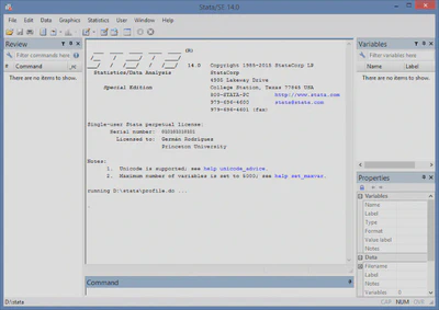
Jane finds data files online with total annual ice cream sales in the 50 largest U.S. cities from 2001-2010 and total numbers of crimes (by type) for the 50 largest U.S. cities from 2001-2010. She gets them as spreadsheets and downloads them to her computer, saving them in her main
Downloadsfolder which includes everything she’s downloaded over the past three years. It probably looks something like this: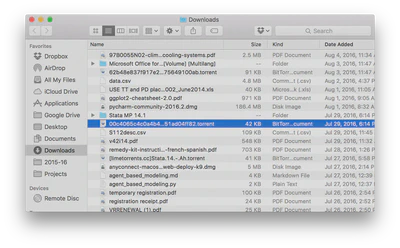
Jane opens the files in Excel.
- Ice cream sales - frozen yogurt is not ice cream. She deletes the column for frozen yogurt sales.
- Crime data - Jane is only interested in violent crime. She deletes all rows pertaining to non-violent offenses.
- Jane saves these modified spreadsheets in a new folder created for this paper.
Jane opens Stata.
- First she imports the ice cream data file using the drop-down menu.
- Next she merges this with the crime data using the drop-down menu. There are some settings she tweaks when she does this, but Jane doesn’t bother to write them down anywhere.
- Then she creates new variables for per capita ice cream sales and per capita crime rates.
- After that, she estimates a linear regression model for the relationship between the two per capita variables.
- Finally she creates a graph plotting the relationship between these two variables.
Jane writes her report in Google Docs.
- Huzzah! She finds a correlation between the two variables. Jane writes up her awesome findings and prepares for her A+.
- The professor wants her results in the paper itself? Darn it. Okay, she copies and pastes her regression results and graph into the paper.
Jane prints her report and turns it in to the professor. Done!
Sally: Using a computational data science workflow
- Sally creates a folder specifically for this project and divides it into subfolders (e.g.
data,graphics,output). - Next she finds data files online with total annual ice cream sales in the 50 largest U.S. cities from 2001-2010 and total numbers of crimes (by type) for the 50 largest U.S. cities from 2001-2010. She writes a program to download these files to the
datasubfolder. - Then Sally writes a program in R that opens each data file and filters/cleans the data to get the necessary variables. She saves the cleaned data as new files in the
datafolder. - Sally writes a separate program which imports the cleaned data files, estimates a regression model, generates a graph, and saves the regression results and graph to the
outputsubfolder. - Sally creates an R Markdown document for her report and analysis. Because R Markdown combines both code and text, the results from step 3 are automatically added into the final report.
- Sally submits the report to the professor. Done!
The value of automation
The professor is impressed with Jane and Sally’s findings, but wants them to verify the results using new data files for ice cream and frozen yogurt sales and crime rates for 2011-2020 before he will determine their grade.
At this point, Jane is greatly hampered by her GUI workflow. She now has to repeat steps 1-5 all over again, but she forgot how she defined violent vs. non-violent crimes. She also no longer has the original frozen yogurt sales data and has to find the original file again somewhere on her computer or online. She has to remember precisely all the menus she entered and all the settings she changed in order to reproduce her findings.
Sally’s computational workflow is much better suited to the professor’s request because it is automated. All Sally needs to do is add the updated data files to the data subfolder, then rewrite her program in step 2 to combine the old and new data files. Next she can simply re-run the programs in steps 3 and 4 with no modifications. The analysis program accepts the new data files without issue and generates the updated regression model estimates and graph. The R Markdown document automatically includes these revised results without any need to modify the code in underlying document.
By automating her workflow, Sally can quickly update her results. Jane has to do all the same work again. Data cleaning alone is a non-trivial challenge for Jane. And the more data files in a project, the more work that has to be done. Sally’s program makes cleaning the data files trivial - if she wants to clean the data again, she simply runs the program again.
Reproducibility
Previously researchers focused on replication - can the results be duplicated in a new study with different data? In science it is difficult to replicate articles and research, in part because authors don’t provide enough information to easily replicate experiments and studies. Institutional biases also exist against replication - no one wants to publish it, and authors don’t like to have their results challenged.
Reproducibility is “the idea that data analyses, and more generally, scientific claims, are published with their data and software code so that others may verify the findings and build upon them.”4 Scholars who implement reproducibility in their projects can quickly and easily reproduce the original results and trace back to determine how they were derived. This easily enables verification and replication, and allows the researcher to precisely replicate his or her analysis. This is extremely important when writing a paper, submiting it to a journal, then coming back months later for a revise and resubmit because you won’t remember how all the code/analysis works together when completing your revisions.
Because Jane forgot how she initially filtered the data files, she cannot replicate her original results, much less update them with the new data. There is no way to definitively prove how she got her initial results. And even if Jane does remember, she still has to do the work of cleaning the data all over again. Sally’s work is reproducible because she still has all the original data files. Any changes to the files, as well as analysis, are created in the programs she wrote. To reproduce her results, all she needs to do is run the programs again. Anyone who wishes to verify her results can implement her code to reproduce them.
Version control
Research projects involve lots of edits and revisions, and not just in the final paper. Researchers make lots of individual decisions when writing programs and conducting analysis. Why filter this set of rows and not this other set? Do I compute traditional or robust standard errors?
To keep track of all of these decisions and modifications, you could save multiple copies of the same file. But this is bad for two reasons.
- When do you decide to create a new version of the file? What do we name this file?
- Why did you create this new version? How can we include this information in a short file name?
Many of you are probably familiar with cloud storage systems like Dropbox or Google Drive. Why not use those to track files in research projects? For one, multiple authors cannot simultaneously edit these files - how do you combine the changes? There is also no record of who made what changes, and you cannot keep annotations describing the changes and why you made them.
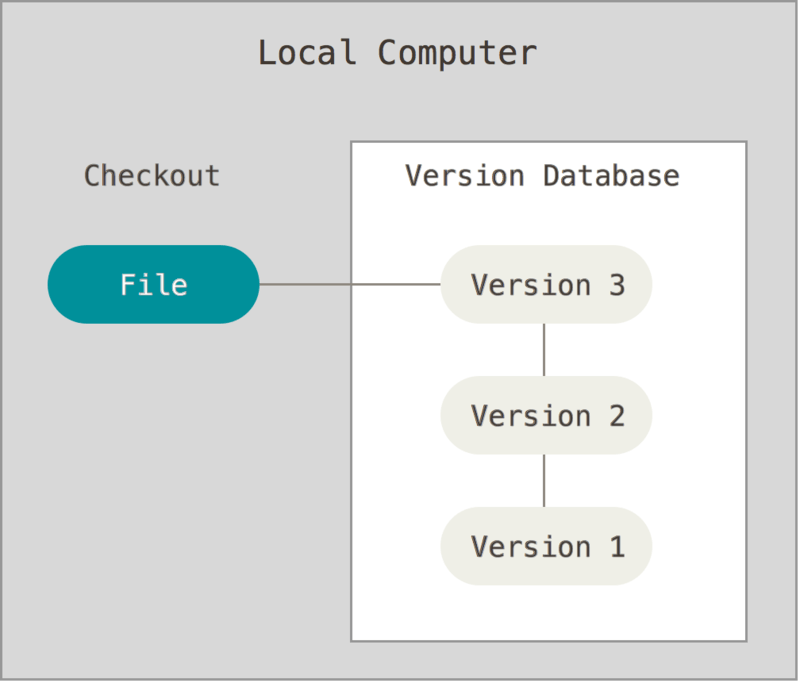
Version control software (VCS) allows us to track all these changes in a detailed and comprehensive manner without resorting to 50 different copies of a file floating around. VCS works by creating a repository on a computer or server which contains all files relevant to a project. Any time you want to modify a file or directory, you check it out. When you are finished, you check it back in. The VCS tracks all changes, when the changes were made, and who made the changes.
If you make a change and realize you don’t want to keep it, you can rollback to a previous version of the repository - or even an individual file - without hassle because the VCS already contains a log of every change. VCS can be implemented locally on a single computer:
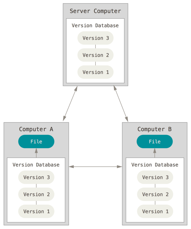
Or in conjunction with remote servers to store backups of your repository:
If Jane wanted to rollback to an earlier implementation of her linear regression model, she’d have to remember exactly what her settings were. However all Sally needs to do is use VCS when she revises her programs. Then to rollback to an earlier model formulation she just needs to find the earlier version of her program which generates that model.
Documentation
Programs include comments which are ignored by the computer but are intended for humans reading the code to understand what it does. So if you decide to ignore frozen yogurt sales, you can include this comment in your code to explain why the program drops that column from the data.
Computer code should also be self-documenting. That is, the code should be comprehensible whenever possible. For example, if you are creating a scatterplot of the relationship between ice cream sales and crime, don’t store it in your code as graph. Instead, give it an intelligible name that intuitively means something, such as icecream_crime_scatterplot or even ic_crime_plot. These records are included directly in the code and should be updated whenever the code is updated.
Comments are not just for other people reading your code, but also for yourself. The goal here is to future-proof your code. That is, future you should be able to open a program and understand what the code does. If you do not include comments and/or write the code in an interpretable way, you will forget how it works.
Badly documented code
This is an example of badly documented code.
library(tidyverse)
library(rtweet)
tml1 <- get_timeline("MeCookieMonster", 3000)
tml2 <- get_timeline("Grover", 3000)
tml3 <- get_timeline("elmo", 3000)
tml4 <- get_timeline("CountVonCount", 3000)
ts_plot(group_by(bind_rows(select(tml1, created_at), select(tml2, created_at), select(tml3, created_at), select(tml4, created_at), .id = "screen_name"), screen_name), by = "months")
- What does this program do?
- What are we using with the
ts_plot()function? - What does
3000refer to?
This program, although it works, is entirely indecipherable unless you are the original author (and even then you may not fully understand it).
Good code
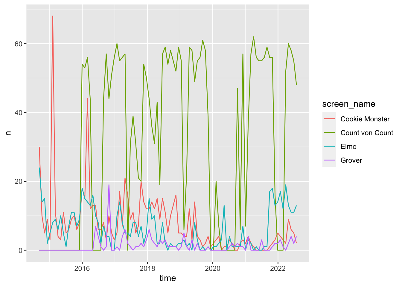
This is a rewritten version of the previous program. Note that it does the exact same thing, but is much more comprehensible.
# get_to_sesame_street.R
# Program to retrieve recent tweets from Sesame Street characters

# load packages for data management and Twitter API
library(tidyverse)
library(rtweet)

# retrieve most recent 3000 tweets of best Sesame Street residents
cookie <- get_timeline(
  user = "MeCookieMonster",
  n = 3000
)

grover <- get_timeline(
  user = "Grover",
  n = 3000
)

elmo <- get_timeline(
  user = "elmo",
  n = 3000
)

count_von_count <- get_timeline(
  user = "CountVonCount",
  n = 3000
)

# combine, group by character, and plot weekly tweet frequency
bind_rows(
  `Cookie Monster` = cookie %>% select(created_at),
  Grover = grover %>% select(created_at),
  Elmo = elmo %>% select(created_at),
  `Count von Count` = count_von_count %>% select(created_at),
  .id = "screen_name"
) %>%
  group_by(screen_name) %>%
  ts_plot(by = "months")
Session Info
sessioninfo::session_info()
## ─ Session info ───────────────────────────────────────────────────────────────
##  setting  value
##  version  R version 4.2.1 (2022-06-23)
##  os       macOS Monterey 12.3
##  system   aarch64, darwin20
##  ui       X11
##  language (EN)
##  collate  en_US.UTF-8
##  ctype    en_US.UTF-8
##  tz       America/New_York
##  date     2022-08-22
##  pandoc   2.18 @ /Applications/RStudio.app/Contents/MacOS/quarto/bin/tools/ (via rmarkdown)
##
## ─ Packages ───────────────────────────────────────────────────────────────────
##  package        * version    date (UTC) lib source
##  assertthat       0.2.1      2019-03-21 [2] CRAN (R 4.2.0)
##  backports        1.4.1      2021-12-13 [2] CRAN (R 4.2.0)
##  bit              4.0.4      2020-08-04 [2] CRAN (R 4.2.0)
##  bit64            4.0.5      2020-08-30 [2] CRAN (R 4.2.0)
##  blogdown         1.10       2022-05-10 [2] CRAN (R 4.2.0)
##  bookdown         0.27       2022-06-14 [2] CRAN (R 4.2.0)
##  broom          * 1.0.0      2022-07-01 [2] CRAN (R 4.2.0)
##  bslib            0.4.0      2022-07-16 [2] CRAN (R 4.2.0)
##  cachem           1.0.6      2021-08-19 [2] CRAN (R 4.2.0)
##  cellranger       1.1.0      2016-07-27 [2] CRAN (R 4.2.0)
##  cli              3.3.0      2022-04-25 [2] CRAN (R 4.2.0)
##  codetools        0.2-18     2020-11-04 [2] CRAN (R 4.2.1)
##  colorspace       2.0-3      2022-02-21 [2] CRAN (R 4.2.0)
##  crayon           1.5.1      2022-03-26 [2] CRAN (R 4.2.0)
##  curl             4.3.2      2021-06-23 [2] CRAN (R 4.2.0)
##  DBI              1.1.3      2022-06-18 [2] CRAN (R 4.2.0)
##  dbplyr           2.2.1      2022-06-27 [2] CRAN (R 4.2.0)
##  digest           0.6.29     2021-12-01 [2] CRAN (R 4.2.0)
##  dplyr          * 1.0.9      2022-04-28 [2] CRAN (R 4.2.0)
##  ellipsis         0.3.2      2021-04-29 [2] CRAN (R 4.2.0)
##  evaluate         0.16       2022-08-09 [1] CRAN (R 4.2.1)
##  fansi            1.0.3      2022-03-24 [2] CRAN (R 4.2.0)
##  farver           2.1.1      2022-07-06 [2] CRAN (R 4.2.0)
##  fastmap          1.1.0      2021-01-25 [2] CRAN (R 4.2.0)
##  forcats        * 0.5.1      2021-01-27 [2] CRAN (R 4.2.0)
##  fs               1.5.2      2021-12-08 [2] CRAN (R 4.2.0)
##  gargle           1.2.0      2021-07-02 [2] CRAN (R 4.2.0)
##  generics         0.1.3      2022-07-05 [2] CRAN (R 4.2.0)
##  ggplot2        * 3.3.6      2022-05-03 [2] CRAN (R 4.2.0)
##  glue             1.6.2      2022-02-24 [2] CRAN (R 4.2.0)
##  googledrive      2.0.0      2021-07-08 [2] CRAN (R 4.2.0)
##  googlesheets4    1.0.0      2021-07-21 [2] CRAN (R 4.2.0)
##  gtable           0.3.0      2019-03-25 [2] CRAN (R 4.2.0)
##  haven            2.5.0      2022-04-15 [2] CRAN (R 4.2.0)
##  here             1.0.1      2020-12-13 [2] CRAN (R 4.2.0)
##  highr            0.9        2021-04-16 [2] CRAN (R 4.2.0)
##  hms              1.1.1      2021-09-26 [2] CRAN (R 4.2.0)
##  htmltools        0.5.3      2022-07-18 [2] CRAN (R 4.2.0)
##  httr             1.4.3      2022-05-04 [2] CRAN (R 4.2.0)
##  jquerylib        0.1.4      2021-04-26 [2] CRAN (R 4.2.0)
##  jsonlite         1.8.0      2022-02-22 [2] CRAN (R 4.2.0)
##  knitr            1.39       2022-04-26 [2] CRAN (R 4.2.0)
##  labeling         0.4.2      2020-10-20 [2] CRAN (R 4.2.0)
##  lifecycle        1.0.1      2021-09-24 [2] CRAN (R 4.2.0)
##  lubridate        1.8.0      2021-10-07 [2] CRAN (R 4.2.0)
##  magrittr         2.0.3      2022-03-30 [2] CRAN (R 4.2.0)
##  modelr           0.1.8      2020-05-19 [2] CRAN (R 4.2.0)
##  munsell          0.5.0      2018-06-12 [2] CRAN (R 4.2.0)
##  palmerpenguins * 0.1.0      2020-07-23 [2] CRAN (R 4.2.0)
##  pillar           1.8.0      2022-07-18 [2] CRAN (R 4.2.0)
##  pkgconfig        2.0.3      2019-09-22 [2] CRAN (R 4.2.0)
##  prettyunits      1.1.1      2020-01-24 [2] CRAN (R 4.2.0)
##  progress         1.2.2      2019-05-16 [2] CRAN (R 4.2.0)
##  purrr          * 0.3.4      2020-04-17 [2] CRAN (R 4.2.0)
##  R6               2.5.1      2021-08-19 [2] CRAN (R 4.2.0)
##  readr          * 2.1.2      2022-01-30 [2] CRAN (R 4.2.0)
##  readxl           1.4.0      2022-03-28 [2] CRAN (R 4.2.0)
##  reprex           2.0.1.9000 2022-08-10 [1] Github (tidyverse/reprex@6d3ad07)
##  rlang            1.0.4      2022-07-12 [2] CRAN (R 4.2.0)
##  rmarkdown        2.14       2022-04-25 [2] CRAN (R 4.2.0)
##  rprojroot        2.0.3      2022-04-02 [2] CRAN (R 4.2.0)
##  rstudioapi       0.13       2020-11-12 [2] CRAN (R 4.2.0)
##  rtweet         * 1.0.2.9005 2022-08-15 [1] Github (ropensci/rtweet@39eecff)
##  rvest            1.0.2      2021-10-16 [2] CRAN (R 4.2.0)
##  sass             0.4.2      2022-07-16 [2] CRAN (R 4.2.0)
##  scales           1.2.0      2022-04-13 [2] CRAN (R 4.2.0)
##  sessioninfo      1.2.2      2021-12-06 [2] CRAN (R 4.2.0)
##  stringi          1.7.8      2022-07-11 [2] CRAN (R 4.2.0)
##  stringr        * 1.4.0      2019-02-10 [2] CRAN (R 4.2.0)
##  tibble         * 3.1.8      2022-07-22 [2] CRAN (R 4.2.0)
##  tidyr          * 1.2.0      2022-02-01 [2] CRAN (R 4.2.0)
##  tidyselect       1.1.2      2022-02-21 [2] CRAN (R 4.2.0)
##  tidyverse      * 1.3.2      2022-07-18 [2] CRAN (R 4.2.0)
##  tzdb             0.3.0      2022-03-28 [2] CRAN (R 4.2.0)
##  utf8             1.2.2      2021-07-24 [2] CRAN (R 4.2.0)
##  vctrs            0.4.1      2022-04-13 [2] CRAN (R 4.2.0)
##  withr            2.5.0      2022-03-03 [2] CRAN (R 4.2.0)
##  xfun             0.31       2022-05-10 [1] CRAN (R 4.2.0)
##  xml2             1.3.3      2021-11-30 [2] CRAN (R 4.2.0)
##  yaml             2.3.5      2022-02-21 [2] CRAN (R 4.2.0)
##
##  [1] /Users/soltoffbc/Library/R/arm64/4.2/library
##  [2] /Library/Frameworks/R.framework/Versions/4.2-arm64/Resources/library
##
## ──────────────────────────────────────────────────────────────────────────────