Drawing vector maps with simple features and ggplot2
library(tidyverse)
library(sf)
library(here)

options(digits = 3)
set.seed(1234)
theme_set(theme_minimal())
Unlike raster image maps, vector maps require you to obtain spatial data files which contain detailed information necessary to draw all the components of a map (e.g. points, lines, polygons). Once you successfully import that data into R, ggplot2 works with simple features data frames to easily generate geospatial visualizations using all the core elements and approaches of ggplot().
Import USA state boundaries
First we will import a spatial data file containing the boundaries of all 50 states in the United States1 using sf::st_read():
usa <- here(
  "static", "data", "census_bureau",
  "cb_2013_us_state_20m", "cb_2013_us_state_20m.shp"
) %>%
  st_read()
## Reading layer `cb_2013_us_state_20m' from data source
##   `/Users/soltoffbc/Projects/Computing for Social Sciences/course-site/static/data/census_bureau/cb_2013_us_state_20m/cb_2013_us_state_20m.shp'
##   using driver `ESRI Shapefile'
## Simple feature collection with 52 features and 9 fields
## Geometry type: MULTIPOLYGON
## Dimension:     XY
## Bounding box:  xmin: -179 ymin: 17.9 xmax: 180 ymax: 71.4
## Geodetic CRS:  NAD83
Draw the boundaries
ggplot2 contains a geometric object specifically for simple feature objects called geom_sf(). This works reasonably well when you need to draw polygons, like our state boundaries. Support for simple features in ggplot2 is under active development, so you may not find adequate support for plotting line or point features. To draw the map, we pass the simple features data frame as the data argument.
ggplot(data = usa) +
  geom_sf()
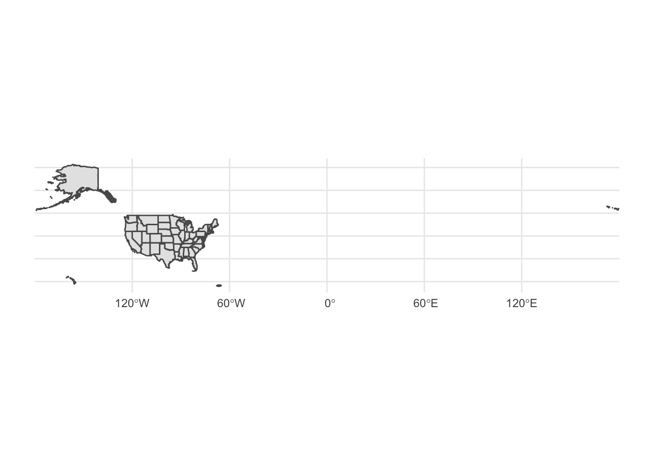
Because simple features data frames are standardized with the geometry column always containing information on the geographic coordinates of the features, we do not need to specify additional parameters for aes(). Notice a problem with the map above: it wastes a lot of space. This is caused by the presence of Alaska and Hawaii in the dataset. The Aleutian Islands cross the the 180th meridian, requiring the map to show the Eastern hemisphere. Likewise, Hawaii is substantially distant from the continental United States.
Plot a subset of a map
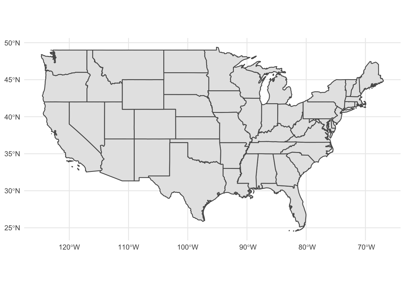
One solution is to plot just the lower 48 states. That is, exclude Alaska and Hawaii, as well as DC and Puerto Rico.2 Because simple features data frames contain one row per feature and in this example a feature is defined as a state, we can use filter() from dplyr to exclude these four states/territories.
usa_48 <- usa %>%
  filter(NAME %in% state.name) %>%
  filter(NAME != "Alaska", NAME != "Hawaii")
usa_48
## Simple feature collection with 48 features and 9 fields
## Geometry type: MULTIPOLYGON
## Dimension:     XY
## Bounding box:  xmin: -125 ymin: 24.5 xmax: -66.9 ymax: 49.4
## Geodetic CRS:  NAD83
## First 10 features:
##    STATEFP  STATENS    AFFGEOID GEOID STUSPS        NAME LSAD    ALAND   AWATER
## 1       01 01779775 0400000US01    01     AL     Alabama   00 1.31e+11 4.59e+09
## 2       05 00068085 0400000US05    05     AR    Arkansas   00 1.35e+11 2.96e+09
## 3       06 01779778 0400000US06    06     CA  California   00 4.03e+11 2.05e+10
## 4       09 01779780 0400000US09    09     CT Connecticut   00 1.25e+10 1.82e+09
## 5       12 00294478 0400000US12    12     FL     Florida   00 1.39e+11 3.14e+10
## 6       13 01705317 0400000US13    13     GA     Georgia   00 1.49e+11 4.95e+09
## 7       16 01779783 0400000US16    16     ID       Idaho   00 2.14e+11 2.40e+09
## 8       17 01779784 0400000US17    17     IL    Illinois   00 1.44e+11 6.20e+09
## 9       18 00448508 0400000US18    18     IN     Indiana   00 9.28e+10 1.54e+09
## 10      20 00481813 0400000US20    20     KS      Kansas   00 2.12e+11 1.35e+09
##                          geometry
## 1  MULTIPOLYGON (((-88.3 30.2,...
## 2  MULTIPOLYGON (((-94.6 36.5,...
## 3  MULTIPOLYGON (((-119 33.5, ...
## 4  MULTIPOLYGON (((-73.7 41.1,...
## 5  MULTIPOLYGON (((-80.7 24.9,...
## 6  MULTIPOLYGON (((-85.6 35, -...
## 7  MULTIPOLYGON (((-117 44.4, ...
## 8  MULTIPOLYGON (((-91.5 40.2,...
## 9  MULTIPOLYGON (((-88.1 37.9,...
## 10 MULTIPOLYGON (((-102 40, -1...
ggplot(data = usa_48) +
  geom_sf()
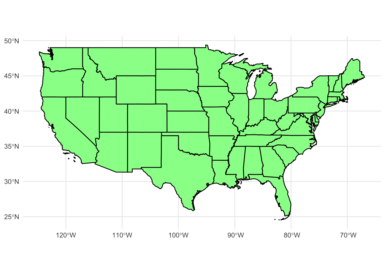
Since the map is a ggplot() object, it can easily be modified like any other ggplot() graph. We could change the color of the map and the borders:
ggplot(data = usa_48) +
  geom_sf(fill = "palegreen", color = "black")
urbanmapr
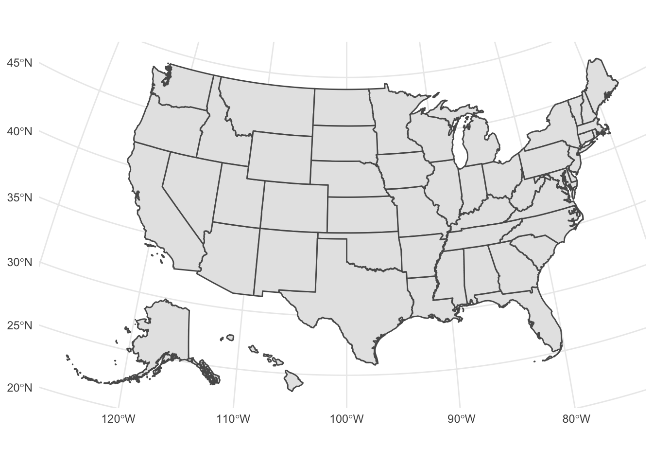
Rather than excluding them entirely, most maps of the United States place Alaska and Hawaii as insets to the south of California. Until recently, in R this was an extremely tedious task that required manually changing the latitude and longitude coordinates for these states to place them in the correct location. Fortunately several packages are now available that have already done the work for you. urbnmapr includes the get_urbn_map() function which returns a simple features data frame which contains adjusted coordinates for Alaska and Hawaii to plot them with the mainland. It can be installed from GitHub using remotes::install_github("UrbanInstitute/urbnmapr").
library(urbnmapr)
states_sf <- get_urbn_map("states", sf = TRUE)

ggplot(data = states_sf) +
  geom_sf()
Add data to the map
Region boundaries serve as the background in geospatial data visualization - so now we need to add data. Some types of geographic data (points and symbols) are overlaid on top of the boundaries, whereas other data (fill) are incorporated into the region layer itself.
Points
Let’s use our crimes data from New York City. crimes is a data frame with each row representing a reported crime in the city. Specifically we will filter the data frame to only examine reported homicides.
crimes <- here("data", "nyc-crimes.csv") %>%
  read_csv()
crimes_homicide <- filter(.data = crimes, ofns_desc == "MURDER & NON-NEGL. MANSLAUGHTER")
crimes_homicide
## # A tibble: 269 × 7
## cmplnt_num boro_nm cmplnt_fr_dt law_cat…¹ ofns_…² latit…³ longi…⁴
## <chr> <chr> <dttm> <chr> <chr> <dbl> <dbl>
## 1 240954923H1 BROOKLYN 1977-12-20 05:00:00 FELONY MURDER… 40.7 -74.0
## 2 245958045H1 BROOKLYN 2001-08-13 04:00:00 FELONY MURDER… 40.7 -73.9
## 3 8101169H6113 MANHATTAN 2005-03-06 05:00:00 FELONY MURDER… 40.8 -73.9
## 4 8101169H6113 MANHATTAN 2005-03-06 05:00:00 FELONY MURDER… 40.8 -73.9
## 5 16631466H8909 BROOKLYN 2006-05-24 04:00:00 FELONY MURDER… 40.7 -73.9
## 6 246056367H1 QUEENS 2015-05-13 04:00:00 FELONY MURDER… 40.6 -73.7
## 7 243507594H1 MANHATTAN 2020-06-19 04:00:00 FELONY MURDER… 40.8 -74.0
## 8 243688124H1 BROOKLYN 2021-01-31 05:00:00 FELONY MURDER… 40.7 -73.9
## 9 240767513H1 BROOKLYN 2021-02-17 05:00:00 FELONY MURDER… 40.6 -74.0
## 10 240767512H1 BROOKLYN 2021-05-24 04:00:00 FELONY MURDER… 40.6 -74.0
## # … with 259 more rows, and abbreviated variable names ¹law_cat_cd, ²ofns_desc,
## # ³latitude, ⁴longitude
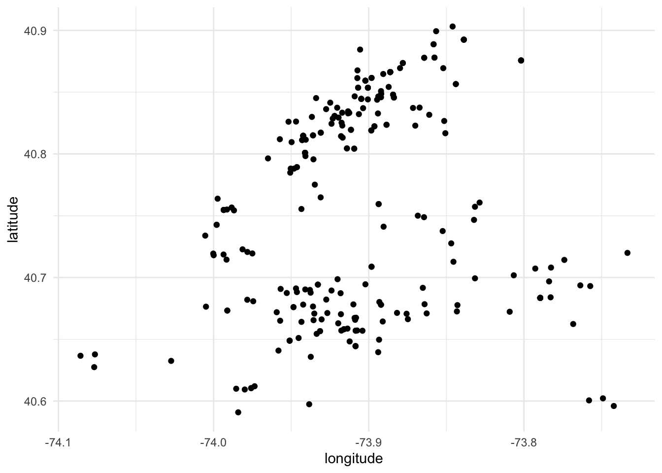
Each crime has it’s geographic location encoded through latitude and longitude. To draw these points on the map, basically we draw a scatterplot with x = longitude and y = latitude. In fact we could simply do that:
ggplot(
  data = crimes_homicide,
  mapping = aes(
    x = longitude,
    y = latitude
  )
) +
  geom_point()
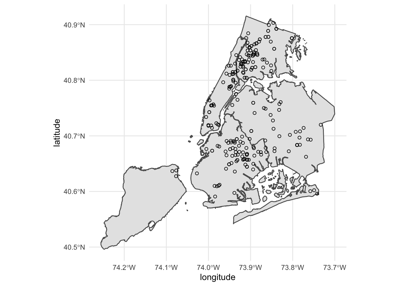
Let’s overlay it with the mapped boroughs:
nyc_json <- st_read(dsn = here("static", "data", "borough-boundaries.geojson"))
## Reading layer `borough-boundaries' from data source
##   `/Users/soltoffbc/Projects/Computing for Social Sciences/course-site/static/data/borough-boundaries.geojson'
##   using driver `GeoJSON'
## Simple feature collection with 5 features and 4 fields
## Geometry type: MULTIPOLYGON
## Dimension:     XY
## Bounding box:  xmin: -74.3 ymin: 40.5 xmax: -73.7 ymax: 40.9
## Geodetic CRS:  WGS 84
ggplot(data = nyc_json) +
  geom_sf() +
  geom_point(
    data = crimes_homicide,
    mapping = aes(
      x = longitude,
      y = latitude
    ),
    shape = 1
  )
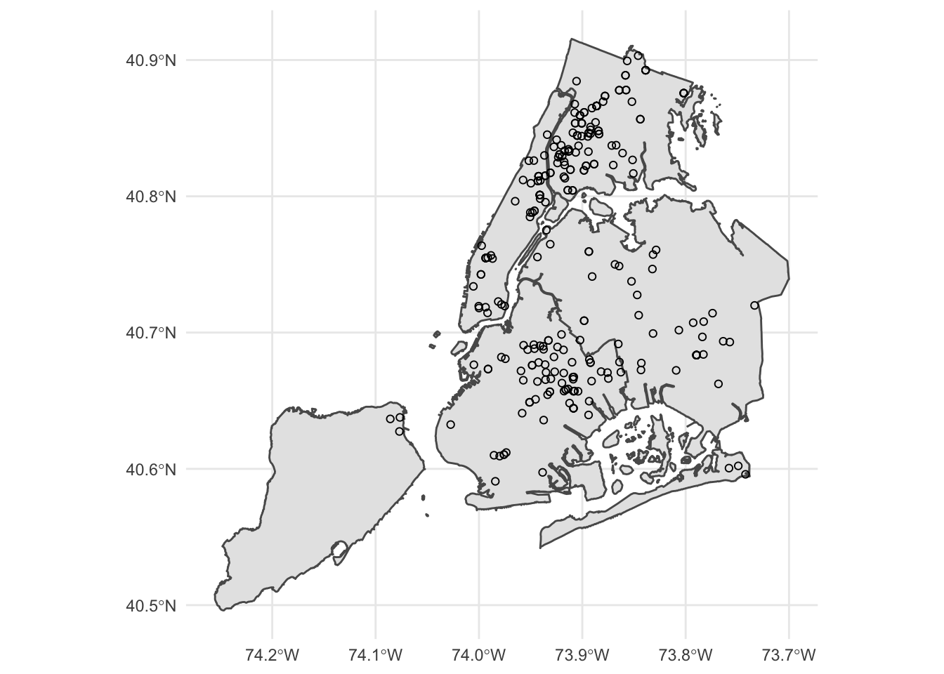
Alternatively, we can use st_as_sf() to convert crimes_homicide to a simple features data frame.
crimes_homicide_sf <- st_as_sf(x = crimes_homicide, coords = c("longitude", "latitude"))
st_crs(crimes_homicide_sf) <- 4326 # set the coordinate reference system
crimes_homicide_sf
## Simple feature collection with 269 features and 5 fields
## Geometry type: POINT
## Dimension: XY
## Bounding box: xmin: -74.1 ymin: 40.6 xmax: -73.7 ymax: 40.9
## Geodetic CRS: WGS 84
## # A tibble: 269 × 6
## cmpln…¹ boro_nm cmplnt_fr_dt law_c…² ofns_…³ geometry
## * <chr> <chr> <dttm> <chr> <chr> <POINT [°]>
## 1 240954… BROOKL… 1977-12-20 05:00:00 FELONY MURDER… (-74 40.7)
## 2 245958… BROOKL… 2001-08-13 04:00:00 FELONY MURDER… (-73.9 40.7)
## 3 810116… MANHAT… 2005-03-06 05:00:00 FELONY MURDER… (-73.9 40.8)
## 4 810116… MANHAT… 2005-03-06 05:00:00 FELONY MURDER… (-73.9 40.8)
## 5 166314… BROOKL… 2006-05-24 04:00:00 FELONY MURDER… (-73.9 40.7)
## 6 246056… QUEENS 2015-05-13 04:00:00 FELONY MURDER… (-73.7 40.6)
## 7 243507… MANHAT… 2020-06-19 04:00:00 FELONY MURDER… (-74 40.8)
## 8 243688… BROOKL… 2021-01-31 05:00:00 FELONY MURDER… (-73.9 40.7)
## 9 240767… BROOKL… 2021-02-17 05:00:00 FELONY MURDER… (-74 40.6)
## 10 240767… BROOKL… 2021-05-24 04:00:00 FELONY MURDER… (-74 40.6)
## # … with 259 more rows, and abbreviated variable names ¹cmplnt_num,
## # ²law_cat_cd, ³ofns_desc
coords tells st_as_sf() which columns contain the geographic coordinates of each airport. To graph the points on the map, we use a second geom_sf()
ggplot() +
  geom_sf(data = nyc_json) +
  geom_sf(
    data = crimes_homicide_sf,
    shape = 1
  )
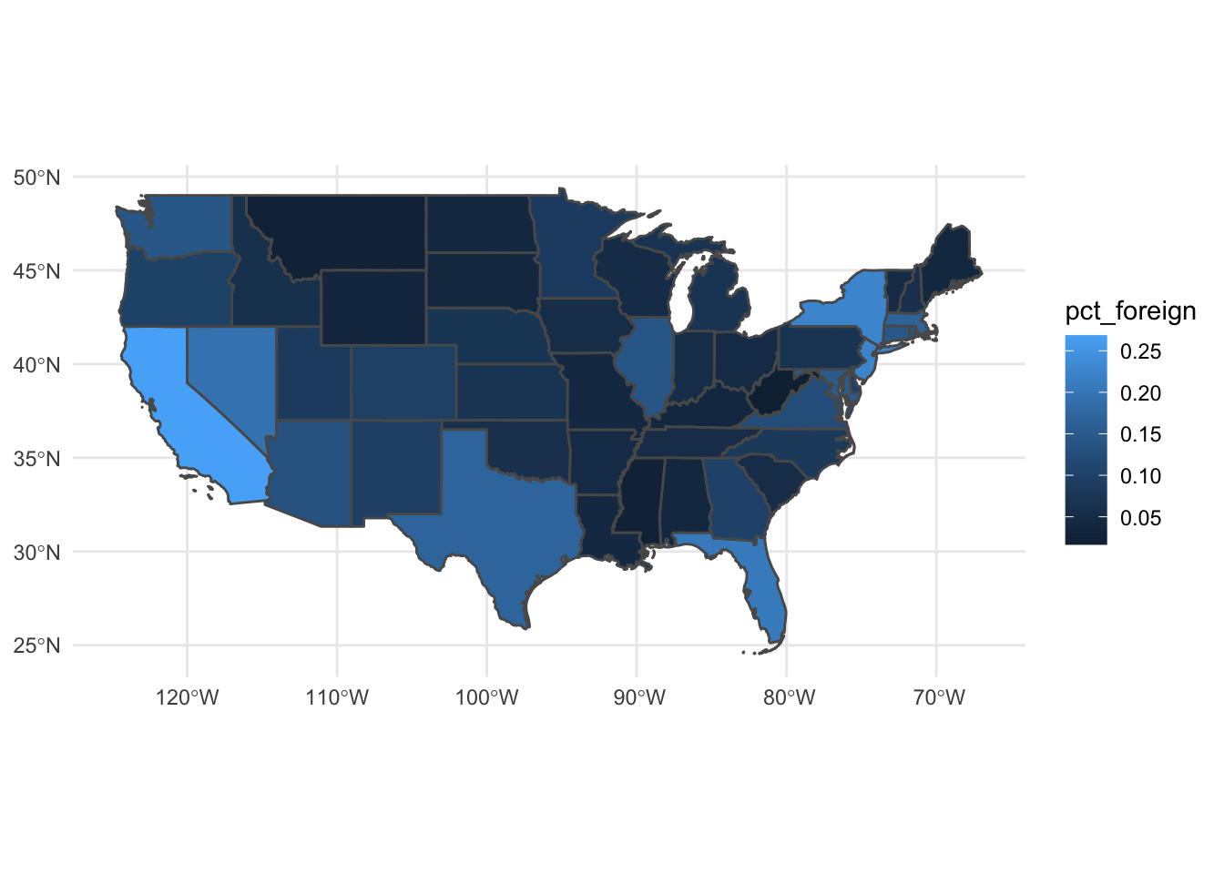
Fill (choropleths)
Choropleth maps encode information by assigning shades of colors to defined areas on a map (e.g. countries, states, counties, zip codes). There are lots of ways to tweak and customize these graphs, which is generally a good idea because remember that color is one of the harder-to-decode channels.
We will continue to use the usa_48 simple features data frame and draw a choropleth for the number of foreign-born individuals in each state. We get those files from the census_bureau folder. Let’s also normalize our measure by the total population to get the rate of foreign-born individuals in the population:
fb_state <- read_csv(file = here("static", "data", "foreign-born.csv"))
fb_state
## # A tibble: 52 × 6
##    GEOID NAME                    total   native  foreign pct_foreign
##    <chr> <chr>                   <dbl>    <dbl>    <dbl>       <dbl>
##  1 01    Alabama               4876250  4703303   172947      0.0355
##  2 02    Alaska                 737068   679401    57667      0.0782
##  3 04    Arizona               7050299  6109648   940651      0.133
##  4 05    Arkansas              2999370  2854323   145047      0.0484
##  5 06    California           39283497 28736287 10547210      0.268
##  6 08    Colorado              5610349  5063836   546513      0.0974
##  7 10    Delaware               957248   865775    91473      0.0956
##  8 11    District of Columbia   692683   597618    95065      0.137
##  9 09    Connecticut           3575074  3054123   520951      0.146
## 10 12    Florida              20901636 16576836  4324800      0.207
## # … with 42 more rows
Join the data
Now that we have our data, we want to draw it on the map. fb_state contains one row per state, as does usa_48. Since there is a one-to-one match between the data frames, we join the data frames together first, then use that single data frame to draw the map. This differs from the approach above for drawing points because a point feature is not the same thing as a polygon feature. That is, there were more airports then there were states. Because the spatial data is stored in a data frame with one row per state, all we need to do is merge the data frames together on a column that uniquely identifies each row in each data frame.
usa_fb <- left_join(x = usa_48, y = fb_state, by = c("STATEFP" = "GEOID", "NAME"))
usa_fb
## Simple feature collection with 48 features and 13 fields
## Geometry type: MULTIPOLYGON
## Dimension:     XY
## Bounding box:  xmin: -125 ymin: 24.5 xmax: -66.9 ymax: 49.4
## Geodetic CRS:  NAD83
## First 10 features:
##    STATEFP  STATENS    AFFGEOID GEOID STUSPS        NAME LSAD    ALAND   AWATER
## 1       01 01779775 0400000US01    01     AL     Alabama   00 1.31e+11 4.59e+09
## 2       05 00068085 0400000US05    05     AR    Arkansas   00 1.35e+11 2.96e+09
## 3       06 01779778 0400000US06    06     CA  California   00 4.03e+11 2.05e+10
## 4       09 01779780 0400000US09    09     CT Connecticut   00 1.25e+10 1.82e+09
## 5       12 00294478 0400000US12    12     FL     Florida   00 1.39e+11 3.14e+10
## 6       13 01705317 0400000US13    13     GA     Georgia   00 1.49e+11 4.95e+09
## 7       16 01779783 0400000US16    16     ID       Idaho   00 2.14e+11 2.40e+09
## 8       17 01779784 0400000US17    17     IL    Illinois   00 1.44e+11 6.20e+09
## 9       18 00448508 0400000US18    18     IN     Indiana   00 9.28e+10 1.54e+09
## 10      20 00481813 0400000US20    20     KS      Kansas   00 2.12e+11 1.35e+09
##       total   native  foreign pct_foreign                       geometry
## 1   4876250  4703303   172947      0.0355 MULTIPOLYGON (((-88.3 30.2,...
## 2   2999370  2854323   145047      0.0484 MULTIPOLYGON (((-94.6 36.5,...
## 3  39283497 28736287 10547210      0.2685 MULTIPOLYGON (((-119 33.5, ...
## 4   3575074  3054123   520951      0.1457 MULTIPOLYGON (((-73.7 41.1,...
## 5  20901636 16576836  4324800      0.2069 MULTIPOLYGON (((-80.7 24.9,...
## 6  10403847  9349973  1053874      0.1013 MULTIPOLYGON (((-85.6 35, -...
## 7   1717750  1615307   102443      0.0596 MULTIPOLYGON (((-117 44.4, ...
## 8  12770631 10973669  1796962      0.1407 MULTIPOLYGON (((-91.5 40.2,...
## 9   6665703  6315781   349922      0.0525 MULTIPOLYGON (((-88.1 37.9,...
## 10  2910652  2702807   207845      0.0714 MULTIPOLYGON (((-102 40, -1...
Draw the map
With the newly combined data frame, use geom_sf() and define the fill aesthetic based on the column in usa_fb you want to visualize.
ggplot(data = usa_fb) +
  geom_sf(mapping = aes(fill = pct_foreign))
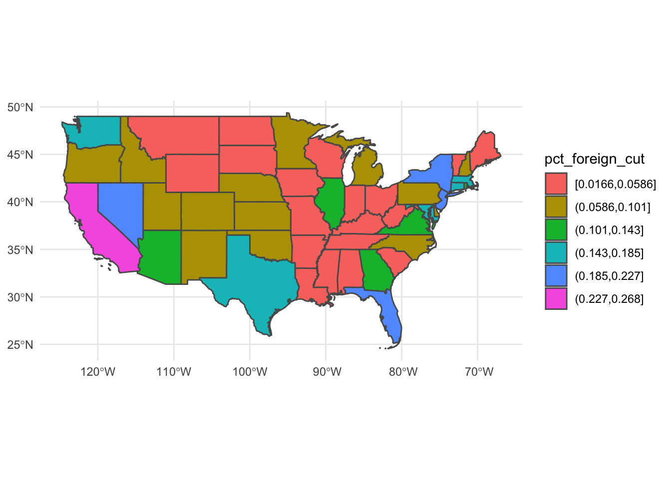
Bin data to discrete intervals
When creating a heatmap with a continuous variable, one must decide whether to keep the variable as continuous or collapse it into a series of bins with discrete colors. While keeping the variable continuous is technically more precise, the human eye cannot usually distinguish between two colors which are very similar to one another. By converting the variable to a discrete variable, you easily distinguish between the different levels. If you decide to convert a continuous variable to a discrete variable, you will need to decide how to do this. While cut() is a base R function for converting continuous variables into discrete values, ggplot2 offers two functions that explicitly define how we want to bin the numeric vector (column).
cut_interval() makes n groups with equal range:
usa_fb %>%
  mutate(pct_foreign_cut = cut_interval(pct_foreign, n = 6)) %>%
  ggplot() +
  geom_sf(aes(fill = pct_foreign_cut))
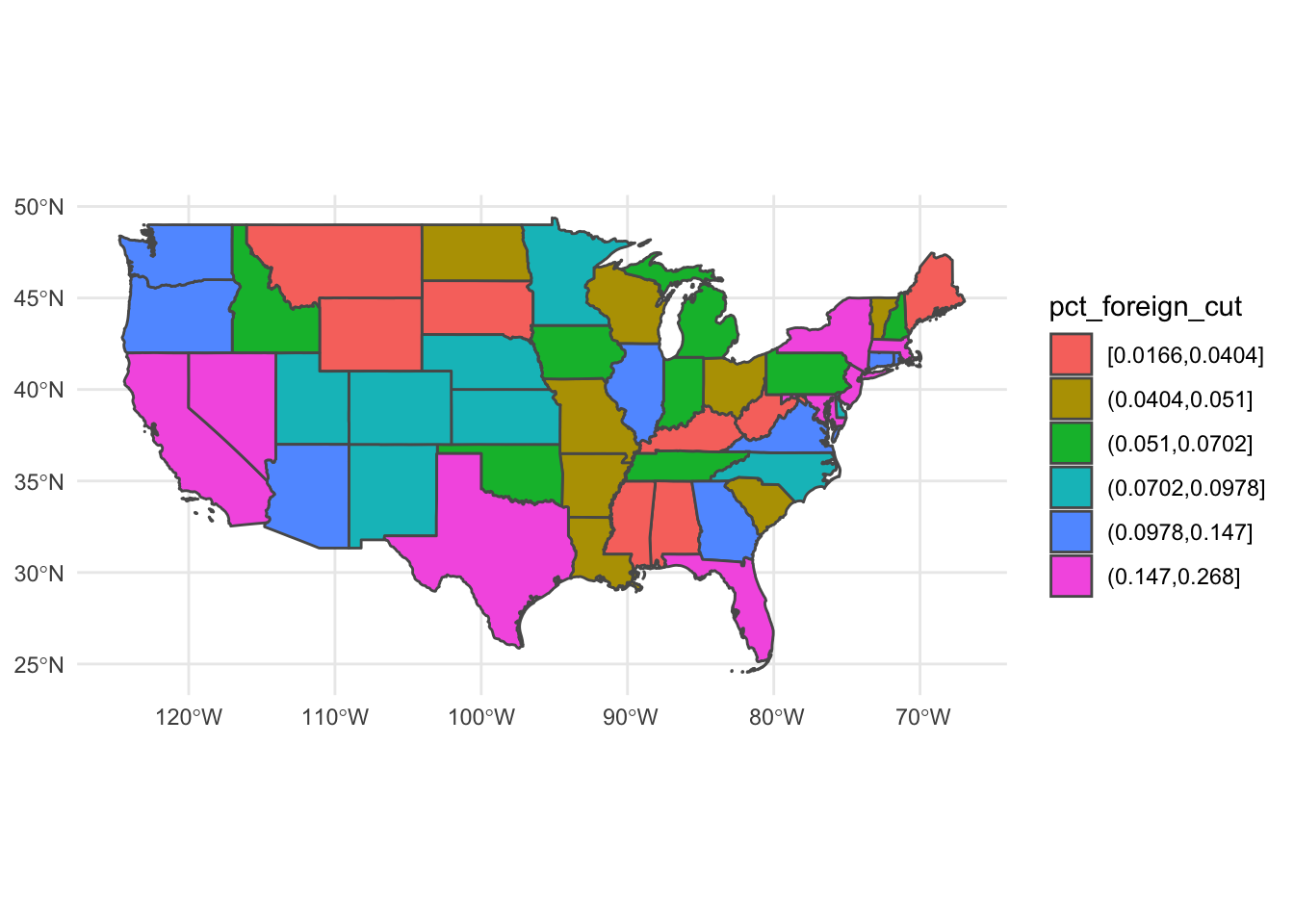
Whereas cut_number() makes n groups with (approximately) equal numbers of observations:
usa_fb %>%
  mutate(pct_foreign_cut = cut_number(pct_foreign, n = 6)) %>%
  ggplot() +
  geom_sf(aes(fill = pct_foreign_cut))
Changing map projection
](https://imgs.xkcd.com/comics/mercator_projection.png)
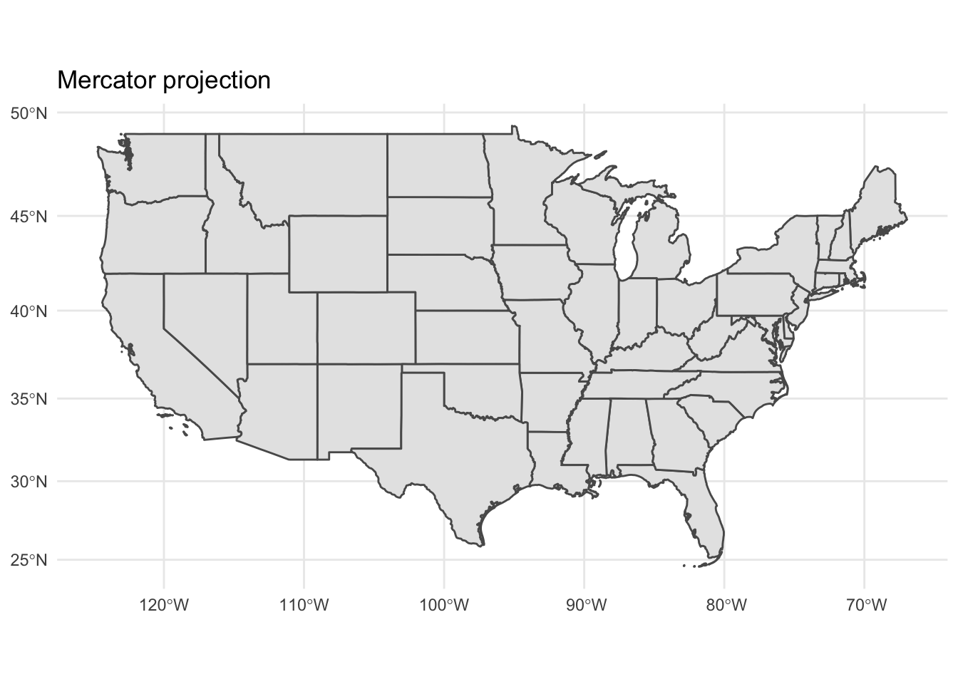
Representing portions of the globe on a flat surface can be challenging. Depending on how you project the map, you can distort or emphasize certain features of the map. Fortunately, ggplot() includes the coord_sf() function which allows us to easily implement different projection methods. In order to implement coordinate transformations, you need to know the coordinate reference system that defines the projection method. The “easiest” approach is to provide what is known as the proj4string that defines the projection method. PROJ4 is a generic coordinate transformation software that allows you to convert between projection methods. If you get really into geospatial analysis and visualization, it is helpful to learn this system.
For our purposes here, proj4string is a character string in R that defines the coordinate system and includes parameters specific to a given coordinate transformation. PROJ4 includes some documentation on common projection methods that can get you started. Some projection methods are relatively simple and require just the name of the projection, like for a Mercator projection ("+proj=merc"):
map_proj_base <- ggplot(data = usa_48) +
  geom_sf()
map_proj_base +
  coord_sf(crs = "+proj=merc") +
  ggtitle("Mercator projection")
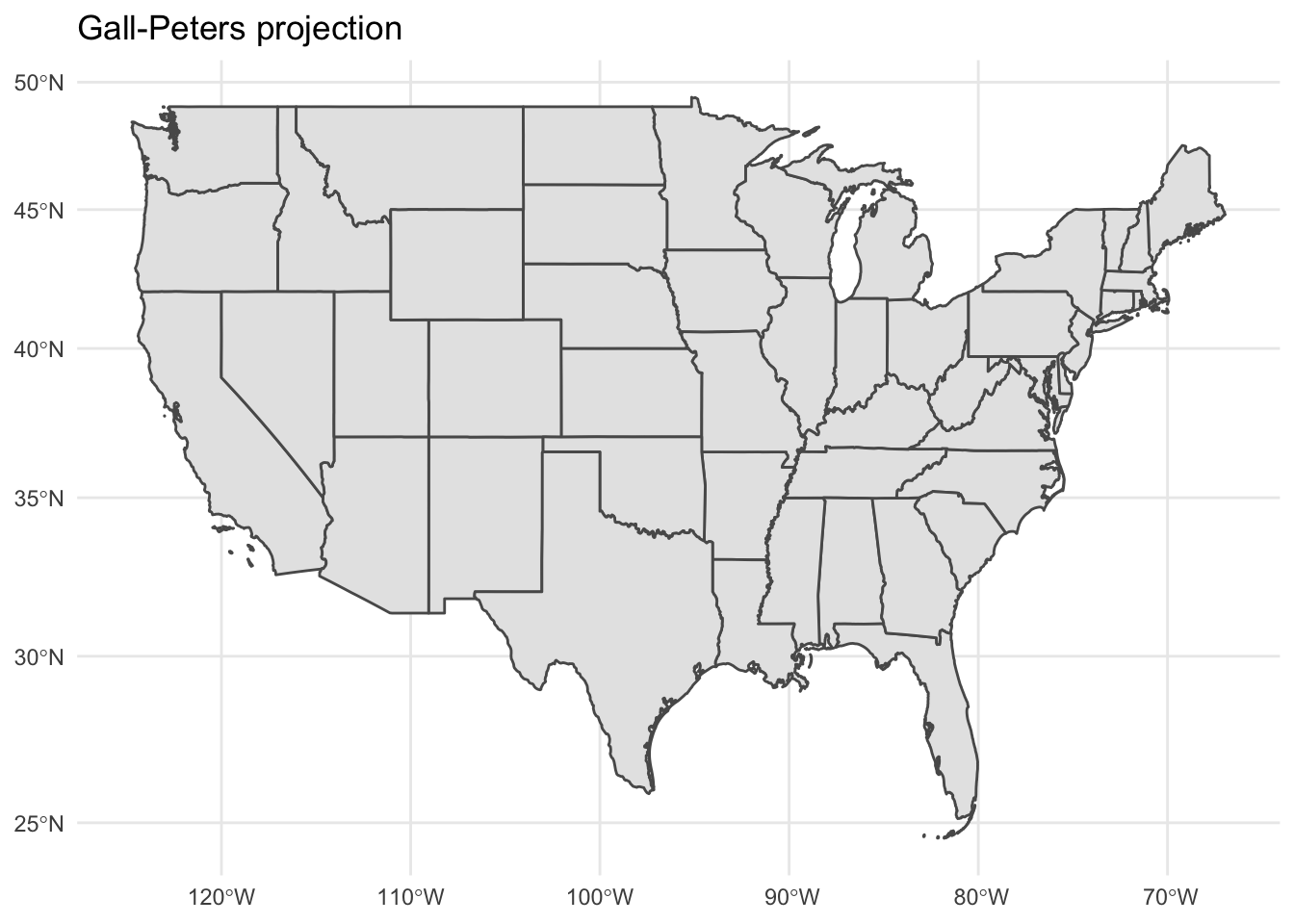
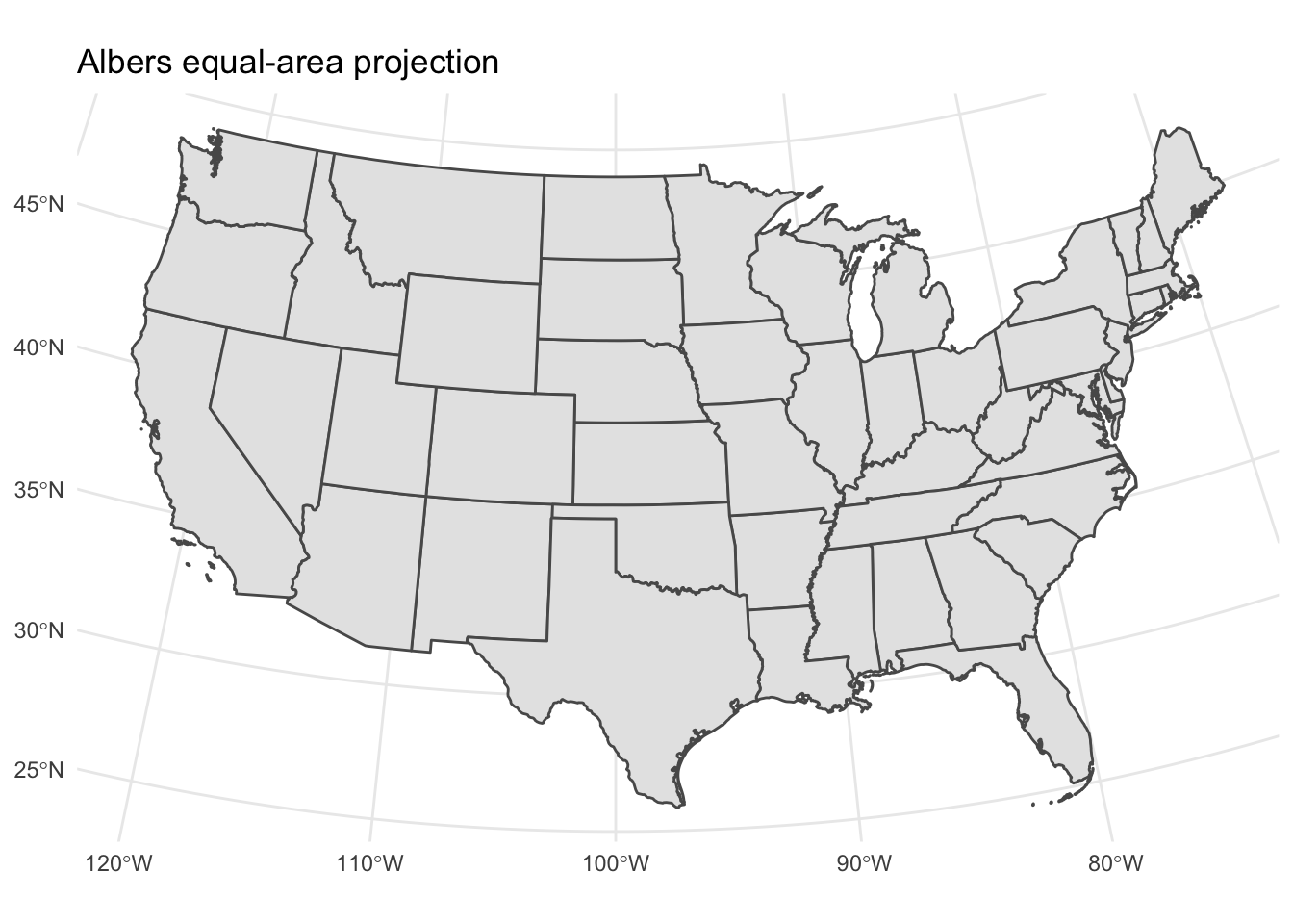
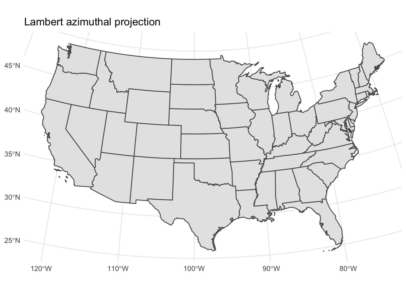
Other coordinate systems require specification of the standard lines, or lines that define areas of the surface of the map that are tangent to the globe. These include Gall-Peters, Albers equal-area, and Lambert azimuthal.
map_proj_base +
  coord_sf(crs = "+proj=cea +lon_0=0 +lat_ts=45") +
  ggtitle("Gall-Peters projection")
map_proj_base +
  coord_sf(crs = "+proj=aea +lat_1=25 +lat_2=50 +lon_0=-100") +
  ggtitle("Albers equal-area projection")
map_proj_base +
  coord_sf(crs = "+proj=laea +lat_0=35 +lon_0=-100") +
  ggtitle("Lambert azimuthal projection")
Session Info
sessioninfo::session_info()
## ─ Session info ───────────────────────────────────────────────────────────────
##  setting  value
##  version  R version 4.2.1 (2022-06-23)
##  os       macOS Monterey 12.3
##  system   aarch64, darwin20
##  ui       X11
##  language (EN)
##  collate  en_US.UTF-8
##  ctype    en_US.UTF-8
##  tz       America/New_York
##  date     2022-10-05
##  pandoc   2.18 @ /Applications/RStudio.app/Contents/MacOS/quarto/bin/tools/ (via rmarkdown)
##
## ─ Packages ───────────────────────────────────────────────────────────────────
##  package       * version    date (UTC) lib source
##  albersusa     * 0.4.1      2022-06-08 [2] Github (hrbrmstr/albersusa@07aa87f)
##  assertthat      0.2.1      2019-03-21 [2] CRAN (R 4.2.0)
##  backports       1.4.1      2021-12-13 [2] CRAN (R 4.2.0)
##  blogdown        1.10       2022-05-10 [2] CRAN (R 4.2.0)
##  bookdown        0.27       2022-06-14 [2] CRAN (R 4.2.0)
##  broom           1.0.0      2022-07-01 [2] CRAN (R 4.2.0)
##  bslib           0.4.0      2022-07-16 [2] CRAN (R 4.2.0)
##  cachem          1.0.6      2021-08-19 [2] CRAN (R 4.2.0)
##  cellranger      1.1.0      2016-07-27 [2] CRAN (R 4.2.0)
##  class           7.3-20     2022-01-16 [2] CRAN (R 4.2.1)
##  classInt        0.4-7      2022-06-10 [2] CRAN (R 4.2.0)
##  cli             3.4.0      2022-09-08 [1] CRAN (R 4.2.0)
##  codetools       0.2-18     2020-11-04 [2] CRAN (R 4.2.1)
##  colorspace      2.0-3      2022-02-21 [2] CRAN (R 4.2.0)
##  crayon          1.5.1      2022-03-26 [2] CRAN (R 4.2.0)
##  DBI             1.1.3      2022-06-18 [2] CRAN (R 4.2.0)
##  dbplyr          2.2.1      2022-06-27 [2] CRAN (R 4.2.0)
##  digest          0.6.29     2021-12-01 [2] CRAN (R 4.2.0)
##  dplyr         * 1.0.9      2022-04-28 [2] CRAN (R 4.2.0)
##  e1071           1.7-11     2022-06-07 [2] CRAN (R 4.2.0)
##  ellipsis        0.3.2      2021-04-29 [2] CRAN (R 4.2.0)
##  evaluate        0.16       2022-08-09 [1] CRAN (R 4.2.1)
##  fansi           1.0.3      2022-03-24 [2] CRAN (R 4.2.0)
##  farver          2.1.1      2022-07-06 [2] CRAN (R 4.2.0)
##  fastmap         1.1.0      2021-01-25 [2] CRAN (R 4.2.0)
##  forcats       * 0.5.1      2021-01-27 [2] CRAN (R 4.2.0)
##  foreign         0.8-82     2022-01-16 [2] CRAN (R 4.2.1)
##  fs              1.5.2      2021-12-08 [2] CRAN (R 4.2.0)
##  gargle          1.2.0      2021-07-02 [2] CRAN (R 4.2.0)
##  generics        0.1.3      2022-07-05 [2] CRAN (R 4.2.0)
##  ggplot2       * 3.3.6      2022-05-03 [2] CRAN (R 4.2.0)
##  glue            1.6.2      2022-02-24 [2] CRAN (R 4.2.0)
##  googledrive     2.0.0      2021-07-08 [2] CRAN (R 4.2.0)
##  googlesheets4   1.0.0      2021-07-21 [2] CRAN (R 4.2.0)
##  gtable          0.3.0      2019-03-25 [2] CRAN (R 4.2.0)
##  haven           2.5.0      2022-04-15 [2] CRAN (R 4.2.0)
##  here          * 1.0.1      2020-12-13 [2] CRAN (R 4.2.0)
##  highr           0.9        2021-04-16 [2] CRAN (R 4.2.0)
##  hms             1.1.1      2021-09-26 [2] CRAN (R 4.2.0)
##  htmltools       0.5.3      2022-07-18 [2] CRAN (R 4.2.0)
##  httr            1.4.3      2022-05-04 [2] CRAN (R 4.2.0)
##  jquerylib       0.1.4      2021-04-26 [2] CRAN (R 4.2.0)
##  jsonlite        1.8.0      2022-02-22 [2] CRAN (R 4.2.0)
##  KernSmooth      2.23-20    2021-05-03 [2] CRAN (R 4.2.1)
##  knitr           1.40       2022-08-24 [1] CRAN (R 4.2.0)
##  lattice         0.20-45    2021-09-22 [2] CRAN (R 4.2.1)
##  lifecycle       1.0.2      2022-09-09 [1] CRAN (R 4.2.0)
##  lubridate       1.8.0      2021-10-07 [2] CRAN (R 4.2.0)
##  magrittr        2.0.3      2022-03-30 [2] CRAN (R 4.2.0)
##  maptools        1.1-4      2022-04-17 [2] CRAN (R 4.2.0)
##  modelr          0.1.8      2020-05-19 [2] CRAN (R 4.2.0)
##  munsell         0.5.0      2018-06-12 [2] CRAN (R 4.2.0)
##  nycflights13  * 1.0.2      2021-04-12 [2] CRAN (R 4.2.0)
##  pillar          1.8.1      2022-08-19 [1] CRAN (R 4.2.0)
##  pkgconfig       2.0.3      2019-09-22 [2] CRAN (R 4.2.0)
##  proxy           0.4-27     2022-06-09 [2] CRAN (R 4.2.0)
##  purrr         * 0.3.4      2020-04-17 [2] CRAN (R 4.2.0)
##  R6              2.5.1      2021-08-19 [2] CRAN (R 4.2.0)
##  Rcpp            1.0.9      2022-07-08 [2] CRAN (R 4.2.0)
##  readr         * 2.1.2      2022-01-30 [2] CRAN (R 4.2.0)
##  readxl          1.4.0      2022-03-28 [2] CRAN (R 4.2.0)
##  reprex          2.0.1.9000 2022-08-10 [1] Github (tidyverse/reprex@6d3ad07)
##  rgdal           1.5-32     2022-05-09 [2] CRAN (R 4.2.0)
##  rgeos           0.5-9      2021-12-15 [2] CRAN (R 4.2.0)
##  rlang           1.0.5      2022-08-31 [1] CRAN (R 4.2.0)
##  rmarkdown       2.14       2022-04-25 [2] CRAN (R 4.2.0)
##  rprojroot       2.0.3      2022-04-02 [2] CRAN (R 4.2.0)
##  rstudioapi      0.13       2020-11-12 [2] CRAN (R 4.2.0)
##  rvest           1.0.2      2021-10-16 [2] CRAN (R 4.2.0)
##  s2              1.1.0      2022-07-18 [2] CRAN (R 4.2.0)
##  sass            0.4.2      2022-07-16 [2] CRAN (R 4.2.0)
##  scales          1.2.0      2022-04-13 [2] CRAN (R 4.2.0)
##  sessioninfo     1.2.2      2021-12-06 [2] CRAN (R 4.2.0)
##  sf            * 1.0-8      2022-07-14 [2] CRAN (R 4.2.0)
##  sp              1.5-0      2022-06-05 [2] CRAN (R 4.2.0)
##  stringi         1.7.8      2022-07-11 [2] CRAN (R 4.2.0)
##  stringr       * 1.4.0      2019-02-10 [2] CRAN (R 4.2.0)
##  tibble        * 3.1.8      2022-07-22 [2] CRAN (R 4.2.0)
##  tidyr         * 1.2.0      2022-02-01 [2] CRAN (R 4.2.0)
##  tidyselect      1.1.2      2022-02-21 [2] CRAN (R 4.2.0)
##  tidyverse     * 1.3.2      2022-07-18 [2] CRAN (R 4.2.0)
##  tzdb            0.3.0      2022-03-28 [2] CRAN (R 4.2.0)
##  units           0.8-0      2022-02-05 [2] CRAN (R 4.2.0)
##  urbnmapr      * 0.0.0.9002 2022-06-08 [2] Github (UrbanInstitute/urbnmapr@ef9f448)
##  utf8            1.2.2      2021-07-24 [2] CRAN (R 4.2.0)
##  vctrs           0.4.1      2022-04-13 [2] CRAN (R 4.2.0)
##  withr           2.5.0      2022-03-03 [2] CRAN (R 4.2.0)
##  wk              0.6.0      2022-01-03 [2] CRAN (R 4.2.0)
##  xfun            0.31       2022-05-10 [1] CRAN (R 4.2.0)
##  xml2            1.3.3      2021-11-30 [2] CRAN (R 4.2.0)
##  yaml            2.3.5      2022-02-21 [2] CRAN (R 4.2.0)
##
##  [1] /Users/soltoffbc/Library/R/arm64/4.2/library
##  [2] /Library/Frameworks/R.framework/Versions/4.2-arm64/Resources/library
##
## ──────────────────────────────────────────────────────────────────────────────