Practice drawing vector maps
library(tidyverse)
library(sf)
library(tidycensus)
library(colorspace)
library(scales)

# useful on MacOS to speed up rendering of geom_sf() objects
if (!identical(getOption("bitmapType"), "cairo") && isTRUE(capabilities()[["cairo"]])) {
  options(bitmapType = "cairo")
}

options(digits = 3)
set.seed(123)
theme_set(theme_minimal())
Run the code below in your console to download this exercise as a set of R scripts.
usethis::use_course("cis-ds/visualize-spatial-ii")
American Community Survey
The U.S. Census Bureau conducts the American Community Survey which gathers detailed information on topics such as demographics, employment, educational attainment, etc. They make a vast portion of their data available through an application programming interface (API), which can be accessed intuitively through R via the tidycensus package. We previously discussed how to use this package to obtain statistical data from the decennial census. However the Census Bureau also has detailed information on political and geographic boundaries which we can combine with their statistical measures to easily construct geospatial visualizations.
Exercise: Visualize income data
- Obtain information on median household income in 2020 for Tompkins County, NY at the tract-level using the ACS. To retrieve the geographic features for each tract, set
geometry = TRUEin your function.
load_variables(year = 2020, dataset = "acs5") to retrieve the list of variables available and search to find the correct variable name.Click for the solution
tompkins_inc <- get_acs(
  state = "NY",
  county = "Tompkins",
  geography = "tract",
  variables = c(medincome = "B19013_001"),
  year = 2020,
  geometry = TRUE,
  output = "wide"
)
tompkins_inc
## Simple feature collection with 26 features and 4 fields
## Geometry type: MULTIPOLYGON
## Dimension:     XY
## Bounding box:  xmin: -76.7 ymin: 42.3 xmax: -76.2 ymax: 42.6
## Geodetic CRS:  NAD83
## First 10 features:
##          GEOID                                         NAME medincomeE
## 1  36109000100    Census Tract 1, Tompkins County, New York      36309
## 2  36109001600   Census Tract 16, Tompkins County, New York      61756
## 3  36109000300    Census Tract 3, Tompkins County, New York         NA
## 4  36109000800    Census Tract 8, Tompkins County, New York      52704
## 5  36109000202 Census Tract 2.02, Tompkins County, New York      20515
## 6  36109000900    Census Tract 9, Tompkins County, New York      71228
## 7  36109001200   Census Tract 12, Tompkins County, New York         NA
## 8  36109000201 Census Tract 2.01, Tompkins County, New York         NA
## 9  36109001400   Census Tract 14, Tompkins County, New York      73818
## 10 36109000600    Census Tract 6, Tompkins County, New York      82756
##    medincomeM                       geometry
## 1        4335 MULTIPOLYGON (((-76.5 42.4,...
## 2        8472 MULTIPOLYGON (((-76.7 42.5,...
## 3          NA MULTIPOLYGON (((-76.5 42.5,...
## 4        9354 MULTIPOLYGON (((-76.5 42.4,...
## 5       15240 MULTIPOLYGON (((-76.5 42.4,...
## 6        9707 MULTIPOLYGON (((-76.6 42.5,...
## 7          NA MULTIPOLYGON (((-76.5 42.4,...
## 8          NA MULTIPOLYGON (((-76.5 42.4,...
## 9       14518 MULTIPOLYGON (((-76.4 42.5,...
## 10      24036 MULTIPOLYGON (((-76.5 42.5,...
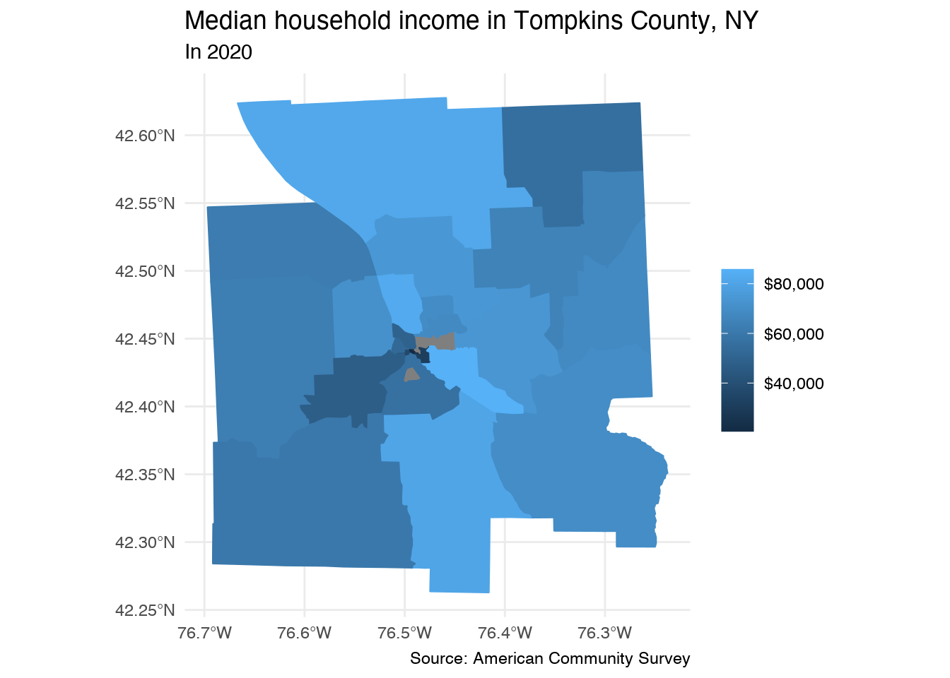
- Draw a choropleth using the median household income data. Use a continuous color gradient to identify each tract’s median household income.
Use the object below to add informative labels to each plot without having to copy-and-paste.
# create reusable labels for each plot
map_labels <- labs(
  title = "Median household income in Tompkins County, NY",
  subtitle = "In 2020",
  color = NULL,
  fill = NULL,
  caption = "Source: American Community Survey"
)
Click for the solution
ggplot(data = tompkins_inc) +
  # use fill and color to avoid gray boundary lines
  geom_sf(aes(fill = medincomeE, color = medincomeE)) +
  # increase interpretability of graph
  scale_color_continuous(labels = label_dollar()) +
  scale_fill_continuous(labels = label_dollar()) +
  map_labels
Exercise: Customize your maps
Use the
viridiscolor palette for the Tompkins County map drawn using the continuous measure.Click for the solution
ggplot(data = tompkins_inc) +
  # use fill and color to avoid gray boundary lines
  geom_sf(aes(fill = medincomeE, color = medincomeE)) +
  # increase interpretability of graph
  scale_fill_continuous_sequential(
    palette = "viridis",
    rev = FALSE,
    aesthetics = c("fill", "color"),
    labels = label_dollar(),
    name = NULL
  ) +
  map_labels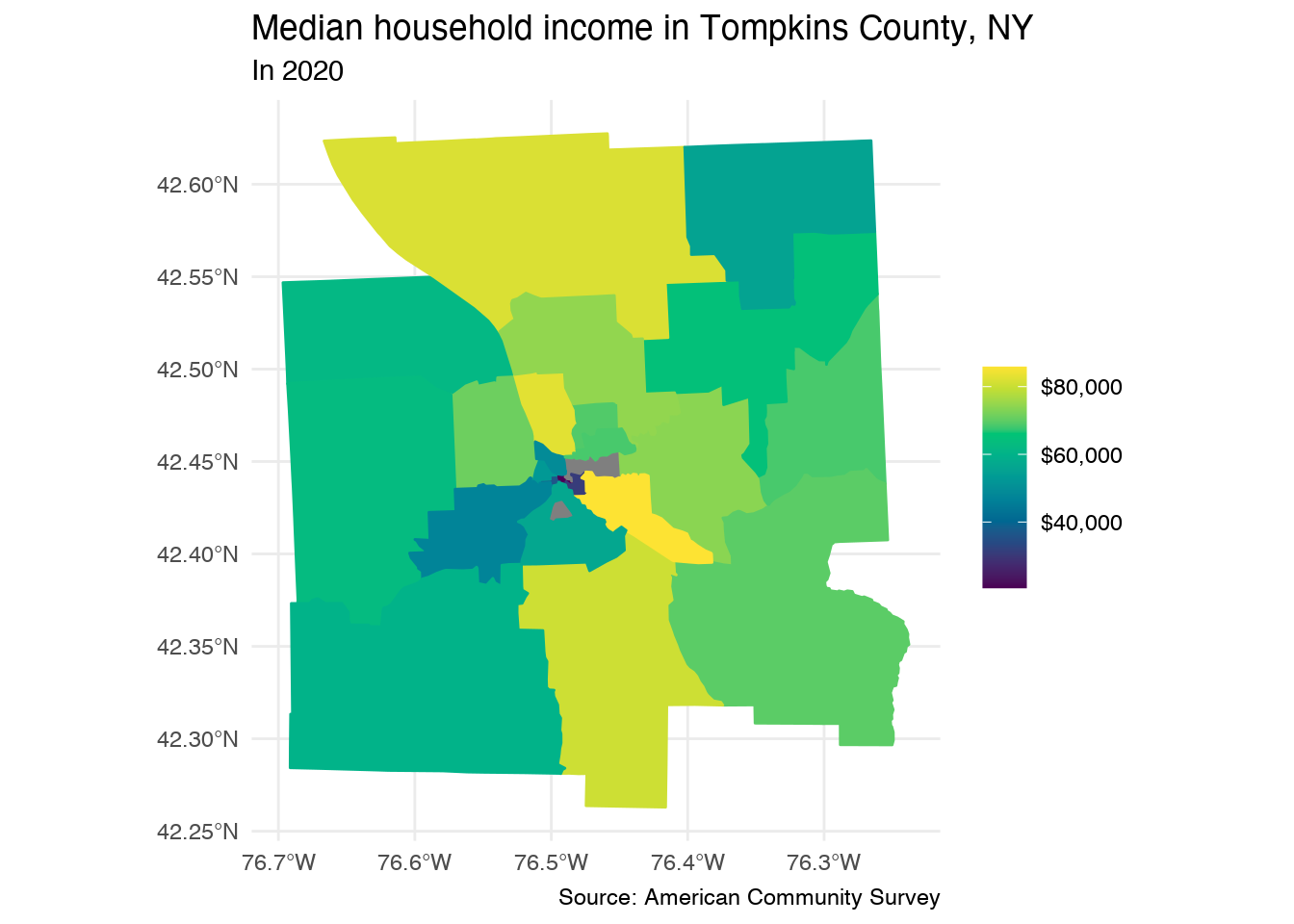
Draw the same choropleth for Tompkins County, but convert median household income into a discrete variable with 6 levels.
Click for the solution
* Using `cut_interval()`:tompkins_inc %>% mutate(inc_cut = cut_interval(medincomeE, n = 6)) %>% ggplot() + # use fill and color to avoid gray boundary lines geom_sf(aes(fill = inc_cut, color = inc_cut)) + # increase interpretability of graph scale_fill_discrete_sequential( palette = "viridis", rev = FALSE, aesthetics = c("fill", "color"), name = NULL ) + map_labels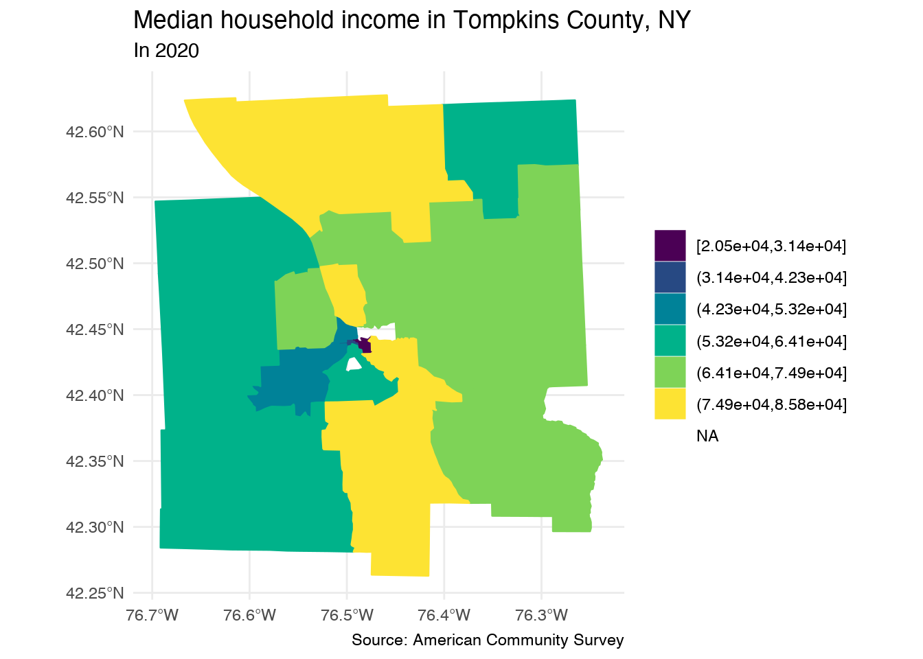
* Using `cut_number()`:tompkins_inc %>% mutate(inc_cut = cut_number(medincomeE, n = 6)) %>% ggplot() + # use fill and color to avoid gray boundary lines geom_sf(aes(fill = inc_cut, color = inc_cut)) + # increase interpretability of graph scale_fill_discrete_sequential( palette = "viridis", rev = FALSE, aesthetics = c("fill", "color"), name = NULL ) + map_labels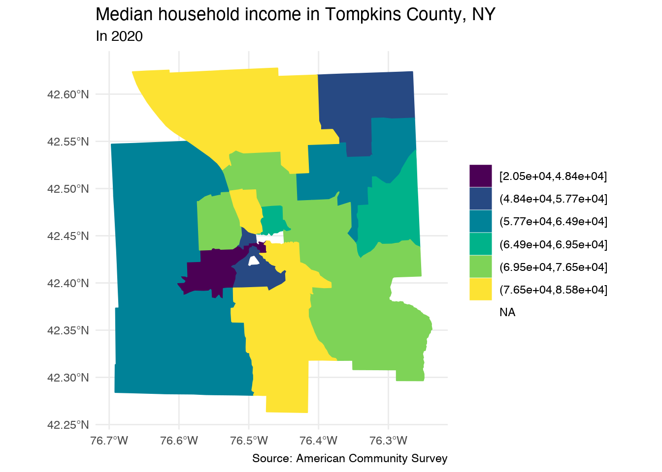
- Using `binned_scale()`# default breaks ggplot(data = tompkins_inc) + geom_sf(mapping = aes(fill = medincomeE, color = medincomeE)) + scale_fill_binned_sequential( palette = "viridis", rev = FALSE, aesthetics = c("fill", "color"), labels = label_dollar() ) + # increase interpretability of graph map_labels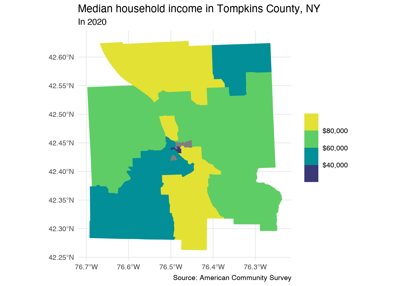
# quintiles
ggplot(data = tompkins_inc) +
  geom_sf(mapping = aes(fill = medincomeE, color = medincomeE)) +
  scale_fill_binned_sequential(
    palette = "viridis",
    rev = FALSE,
    aesthetics = c("fill", "color"),
    n.breaks = 4, nice.breaks = FALSE,
    labels = label_dollar()
  ) +
  # increase interpretability of graph
  map_labels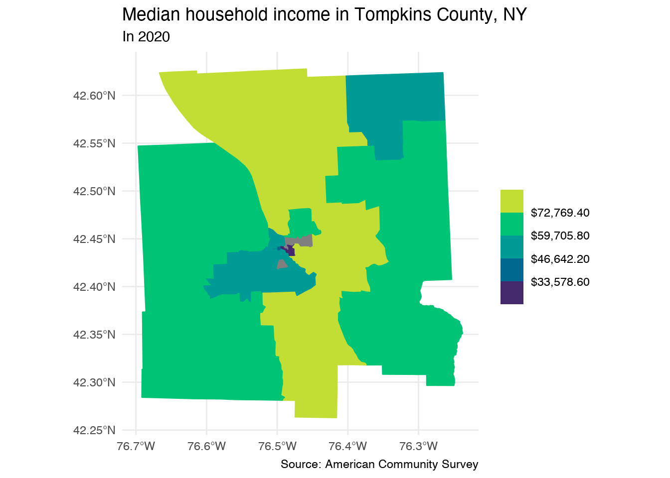
Session Info
sessioninfo::session_info()
## ─ Session info ───────────────────────────────────────────────────────────────
##  setting  value
##  version  R version 4.2.1 (2022-06-23)
##  os       macOS Monterey 12.3
##  system   aarch64, darwin20
##  ui       X11
##  language (EN)
##  collate  en_US.UTF-8
##  ctype    en_US.UTF-8
##  tz       America/New_York
##  date     2022-10-05
##  pandoc   2.18 @ /Applications/RStudio.app/Contents/MacOS/quarto/bin/tools/ (via rmarkdown)
##
## ─ Packages ───────────────────────────────────────────────────────────────────
##  package       * version    date (UTC) lib source
##  assertthat      0.2.1      2019-03-21 [2] CRAN (R 4.2.0)
##  backports       1.4.1      2021-12-13 [2] CRAN (R 4.2.0)
##  blogdown        1.10       2022-05-10 [2] CRAN (R 4.2.0)
##  bookdown        0.27       2022-06-14 [2] CRAN (R 4.2.0)
##  broom           1.0.0      2022-07-01 [2] CRAN (R 4.2.0)
##  bslib           0.4.0      2022-07-16 [2] CRAN (R 4.2.0)
##  cachem          1.0.6      2021-08-19 [2] CRAN (R 4.2.0)
##  cellranger      1.1.0      2016-07-27 [2] CRAN (R 4.2.0)
##  class           7.3-20     2022-01-16 [2] CRAN (R 4.2.1)
##  classInt        0.4-7      2022-06-10 [2] CRAN (R 4.2.0)
##  cli             3.4.0      2022-09-08 [1] CRAN (R 4.2.0)
##  codetools       0.2-18     2020-11-04 [2] CRAN (R 4.2.1)
##  colorspace    * 2.0-3      2022-02-21 [2] CRAN (R 4.2.0)
##  crayon          1.5.1      2022-03-26 [2] CRAN (R 4.2.0)
##  curl            4.3.2      2021-06-23 [2] CRAN (R 4.2.0)
##  DBI             1.1.3      2022-06-18 [2] CRAN (R 4.2.0)
##  dbplyr          2.2.1      2022-06-27 [2] CRAN (R 4.2.0)
##  digest          0.6.29     2021-12-01 [2] CRAN (R 4.2.0)
##  dplyr         * 1.0.9      2022-04-28 [2] CRAN (R 4.2.0)
##  e1071           1.7-11     2022-06-07 [2] CRAN (R 4.2.0)
##  ellipsis        0.3.2      2021-04-29 [2] CRAN (R 4.2.0)
##  evaluate        0.16       2022-08-09 [1] CRAN (R 4.2.1)
##  fansi           1.0.3      2022-03-24 [2] CRAN (R 4.2.0)
##  farver          2.1.1      2022-07-06 [2] CRAN (R 4.2.0)
##  fastmap         1.1.0      2021-01-25 [2] CRAN (R 4.2.0)
##  forcats       * 0.5.1      2021-01-27 [2] CRAN (R 4.2.0)
##  foreign         0.8-82     2022-01-16 [2] CRAN (R 4.2.1)
##  fs              1.5.2      2021-12-08 [2] CRAN (R 4.2.0)
##  gargle          1.2.0      2021-07-02 [2] CRAN (R 4.2.0)
##  generics        0.1.3      2022-07-05 [2] CRAN (R 4.2.0)
##  ggplot2       * 3.3.6      2022-05-03 [2] CRAN (R 4.2.0)
##  glue            1.6.2      2022-02-24 [2] CRAN (R 4.2.0)
##  googledrive     2.0.0      2021-07-08 [2] CRAN (R 4.2.0)
##  googlesheets4   1.0.0      2021-07-21 [2] CRAN (R 4.2.0)
##  gridExtra       2.3        2017-09-09 [2] CRAN (R 4.2.0)
##  gtable          0.3.0      2019-03-25 [2] CRAN (R 4.2.0)
##  haven           2.5.0      2022-04-15 [2] CRAN (R 4.2.0)
##  here            1.0.1      2020-12-13 [2] CRAN (R 4.2.0)
##  highr           0.9        2021-04-16 [2] CRAN (R 4.2.0)
##  hms             1.1.1      2021-09-26 [2] CRAN (R 4.2.0)
##  htmltools       0.5.3      2022-07-18 [2] CRAN (R 4.2.0)
##  httr            1.4.3      2022-05-04 [2] CRAN (R 4.2.0)
##  jquerylib       0.1.4      2021-04-26 [2] CRAN (R 4.2.0)
##  jsonlite        1.8.0      2022-02-22 [2] CRAN (R 4.2.0)
##  KernSmooth      2.23-20    2021-05-03 [2] CRAN (R 4.2.1)
##  knitr           1.40       2022-08-24 [1] CRAN (R 4.2.0)
##  labeling        0.4.2      2020-10-20 [2] CRAN (R 4.2.0)
##  lattice         0.20-45    2021-09-22 [2] CRAN (R 4.2.1)
##  lifecycle       1.0.2      2022-09-09 [1] CRAN (R 4.2.0)
##  lubridate       1.8.0      2021-10-07 [2] CRAN (R 4.2.0)
##  magrittr        2.0.3      2022-03-30 [2] CRAN (R 4.2.0)
##  maptools        1.1-4      2022-04-17 [2] CRAN (R 4.2.0)
##  modelr          0.1.8      2020-05-19 [2] CRAN (R 4.2.0)
##  munsell         0.5.0      2018-06-12 [2] CRAN (R 4.2.0)
##  pillar          1.8.1      2022-08-19 [1] CRAN (R 4.2.0)
##  pkgconfig       2.0.3      2019-09-22 [2] CRAN (R 4.2.0)
##  proxy           0.4-27     2022-06-09 [2] CRAN (R 4.2.0)
##  purrr         * 0.3.4      2020-04-17 [2] CRAN (R 4.2.0)
##  R6              2.5.1      2021-08-19 [2] CRAN (R 4.2.0)
##  rappdirs        0.3.3      2021-01-31 [2] CRAN (R 4.2.0)
##  Rcpp            1.0.9      2022-07-08 [2] CRAN (R 4.2.0)
##  readr         * 2.1.2      2022-01-30 [2] CRAN (R 4.2.0)
##  readxl          1.4.0      2022-03-28 [2] CRAN (R 4.2.0)
##  reprex          2.0.1.9000 2022-08-10 [1] Github (tidyverse/reprex@6d3ad07)
##  rgdal           1.5-32     2022-05-09 [2] CRAN (R 4.2.0)
##  rlang           1.0.5      2022-08-31 [1] CRAN (R 4.2.0)
##  rmarkdown       2.14       2022-04-25 [2] CRAN (R 4.2.0)
##  rprojroot       2.0.3      2022-04-02 [2] CRAN (R 4.2.0)
##  rstudioapi      0.13       2020-11-12 [2] CRAN (R 4.2.0)
##  rvest           1.0.2      2021-10-16 [2] CRAN (R 4.2.0)
##  s2              1.1.0      2022-07-18 [2] CRAN (R 4.2.0)
##  sass            0.4.2      2022-07-16 [2] CRAN (R 4.2.0)
##  scales        * 1.2.0      2022-04-13 [2] CRAN (R 4.2.0)
##  sessioninfo     1.2.2      2021-12-06 [2] CRAN (R 4.2.0)
##  sf            * 1.0-8      2022-07-14 [2] CRAN (R 4.2.0)
##  sp              1.5-0      2022-06-05 [2] CRAN (R 4.2.0)
##  stringi         1.7.8      2022-07-11 [2] CRAN (R 4.2.0)
##  stringr       * 1.4.0      2019-02-10 [2] CRAN (R 4.2.0)
##  tibble        * 3.1.8      2022-07-22 [2] CRAN (R 4.2.0)
##  tidycensus    * 1.2.2      2022-06-03 [2] CRAN (R 4.2.0)
##  tidyr         * 1.2.0      2022-02-01 [2] CRAN (R 4.2.0)
##  tidyselect      1.1.2      2022-02-21 [2] CRAN (R 4.2.0)
##  tidyverse     * 1.3.2      2022-07-18 [2] CRAN (R 4.2.0)
##  tigris          1.6.1      2022-06-03 [2] CRAN (R 4.2.0)
##  tzdb            0.3.0      2022-03-28 [2] CRAN (R 4.2.0)
##  units           0.8-0      2022-02-05 [2] CRAN (R 4.2.0)
##  utf8            1.2.2      2021-07-24 [2] CRAN (R 4.2.0)
##  uuid            1.1-0      2022-04-19 [2] CRAN (R 4.2.0)
##  vctrs           0.4.1      2022-04-13 [2] CRAN (R 4.2.0)
##  viridis       * 0.6.2      2021-10-13 [2] CRAN (R 4.2.0)
##  viridisLite   * 0.4.0      2021-04-13 [2] CRAN (R 4.2.0)
##  withr           2.5.0      2022-03-03 [2] CRAN (R 4.2.0)
##  wk              0.6.0      2022-01-03 [2] CRAN (R 4.2.0)
##  xfun            0.31       2022-05-10 [1] CRAN (R 4.2.0)
##  xml2            1.3.3      2021-11-30 [2] CRAN (R 4.2.0)
##  yaml            2.3.5      2022-02-21 [2] CRAN (R 4.2.0)
##
##  [1] /Users/soltoffbc/Library/R/arm64/4.2/library
##  [2] /Library/Frameworks/R.framework/Versions/4.2-arm64/Resources/library
##
## ──────────────────────────────────────────────────────────────────────────────