Importing spatial data files using sf
library(tidyverse)
library(sf)
library(here)

options(digits = 3)
set.seed(1234)
theme_set(theme_minimal())
Rather than storing spatial data as raster image files which are not easily modifiable, we can instead store spatial data as vector files. Vector files store the underlying geographical features (e.g. points, lines, polygons) as numerical data which software such as R can import and use to draw a map.
There are many popular file formats for storing spatial data. Here we will look at two common file types, shapefiles and GeoJSON.
Shapefile
Shapefiles are a commonly supported file type for spatial data dating back to the early 1990s. Proprietary software for geographic information systems (GIS) such as ArcGIS pioneered this format and helps maintain its continued usage. A shapefile encodes points, lines, and polygons in geographic space, and is actually a set of files. Shapefiles appear with a .shp extension, sometimes with accompanying files ending in .dbf and .prj.
.shpstores the geographic coordinates of the geographic features (e.g. country, state, county).dbfstores data associated with the geographic features (e.g. unemployment rate, crime rates, percentage of votes cast for Donald Trump).prjstores information about the projection of the coordinates in the shapefile
When importing a shapefile, you need to ensure all the files are in the same folder. For example, here is the structure of the Census Bureau’s 2013 state boundaries shapefile:
## -- cb_2013_us_county_20m.dbf
## -- cb_2013_us_county_20m.prj
## -- cb_2013_us_county_20m.shp
## -- cb_2013_us_county_20m.shp.iso.xml
## -- cb_2013_us_county_20m.shp.xml
## -- cb_2013_us_county_20m.shx
## -- county_20m.ea.iso.xml
This is the complete shapefile. If any of these files are missing, you will get an error importing your shapefile:
## Error in CPL_read_ogr(dsn, layer, query, as.character(options), quiet, : Open failed.
GeoJSON
GeoJSON is a newer format for encoding a variety of geographical data structures using the JavaScript Object Notation (JSON) file format. JSON formatted data is frequently used in web development and services. We will explore it in more detail when we get to collecting data from the web. An example of a GeoJSON file is below:
{
  "type": "Feature",
  "geometry": {
    "type": "Point",
    "coordinates": [125.6, 10.1]
  },
  "properties": {
    "name": "Dinagat Islands"
  }
}
GeoJSON files are plain text files and can contain many different types of geometric features.
Simple features
There are a crap ton of packages for R that allow you to interact with shapefiles and spatial data. Here we will focus on a modern package for reading and transforming spatial data in a tidy format.
Simple features or simple feature access refers to a formal standard that describes how objects in the real world can be represented in computers, with emphasis on the spatial geometry of these objects. It also describes how such objects can be stored in and retrieved from databases, and which geometrical operations should be defined for them.
The standard is widely implemented in spatial databases (such as PostGIS), commercial GIS (e.g., ESRI ArcGIS) and forms the vector data basis for libraries such as GDAL. A subset of simple features forms the GeoJSON standard.
R has well-supported classes for storing spatial data (sp) and interfacing to the above mentioned environments (rgdal, rgeos), but has so far lacked a complete implementation of simple features, making conversions at times convoluted, inefficient or incomplete. The sf package tries to fill this gap.
What is a feature?
A feature is a thing or an object in the real world. Often features will consist of a set of features. For instance, a tree can be a feature but a set of trees can form a forest which is itself a feature. Features have geometry describing where on Earth the feature is located. They also have attributes, which describe other properties of the feature.
Dimensions
All geometries are composed of points. Points are coordinates in a 2-, 3- or 4-dimensional space. All points in a geometry have the same dimensionality. In addition to X and Y coordinates, there are two optional additional dimensions:
- a Z coordinate, denoting altitude
- an M coordinate (rarely used), denoting some measure that is associated with the point, rather than with the feature as a whole (in which case it would be a feature attribute); examples could be time of measurement, or measurement error of the coordinates
The four possible cases then are:
- two-dimensional points refer to x and y, easting and northing, or longitude and latitude, we refer to them as XY
- three-dimensional points as XYZ
- three-dimensional points as XYM
- four-dimensional points as XYZM (the third axis is Z, fourth M)
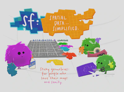
Simple feature geometry types
](/media/simple-features_hu6d3011b6c6c47e09fd746f8649db6ee6_31525_b9d34f136166ff432922c565a7d91e4c.webp)
The following seven simple feature types are the most common, and are for instance the only ones used for GeoJSON:
| type | description |
|---|---|
POINT | zero-dimensional geometry containing a single point |
LINESTRING | sequence of points connected by straight, non-self intersecting line pieces; one-dimensional geometry |
POLYGON | geometry with a positive area (two-dimensional); sequence of points form a closed, non-self intersecting ring; the first ring denotes the exterior ring, zero or more subsequent rings denote holes in this exterior ring |
MULTIPOINT | set of points; a MULTIPOINT is simple if no two Points in the MULTIPOINT are equal |
MULTILINESTRING | set of linestrings |
MULTIPOLYGON | set of polygons |
GEOMETRYCOLLECTION | set of geometries of any type except GEOMETRYCOLLECTION |
Coordinate reference system
Coordinates can only be placed on the Earth’s surface when their coordinate reference system (CRS) is known; this may be an spheroid CRS such as WGS84, a projected, two-dimensional (Cartesian) CRS such as a UTM zone or Web Mercator, or a CRS in three-dimensions, or including time. Similarly, M-coordinates need an attribute reference system, e.g. a measurement unit.
Simple features in R
sf stores simple features as basic R data structures (lists, matrix, vectors, etc.). The typical data structure stores geometric and feature attributes as a data frame with one row per feature. However since feature geometries are not single-valued, they are put in a list-column with each list element holding the simple feature geometry of that feature.
Importing spatial data using sf
st_read() imports a spatial data file and converts it to a simple feature data frame. Here we import a shapefile containing the spatial boundaries of each borough in New York City.
nyc_shape <- here("static", "data", "borough-boundaries") %>%
  st_read()
## Reading layer `geo_export_6fd95df5-1136-4829-8f2d-9cb5d1cc2222' from data source `/Users/soltoffbc/Projects/Computing for Social Sciences/course-site/static/data/borough-boundaries'
##   using driver `ESRI Shapefile'
## Simple feature collection with 5 features and 4 fields
## Geometry type: MULTIPOLYGON
## Dimension:     XY
## Bounding box:  xmin: -74.3 ymin: 40.5 xmax: -73.7 ymax: 40.9
## Geodetic CRS:  WGS84(DD)
The short report printed gives the file name, mentions that there are 5 features (records, represented as rows) and 5 fields (attributes, represented as columns), states that the spatial data file is a MULTIPOLYGON, provides the bounding box coordinates, and identifies the projection method (which we will discuss later). If we print the first rows of nyc_shape:
nyc_shape
## Simple feature collection with 5 features and 4 fields
## Geometry type: MULTIPOLYGON
## Dimension:     XY
## Bounding box:  xmin: -74.3 ymin: 40.5 xmax: -73.7 ymax: 40.9
## Geodetic CRS:  WGS84(DD)
##   boro_code     boro_name shape_area shape_leng                       geometry
## 1         5 Staten Island   1.62e+09     325924 MULTIPOLYGON (((-74.1 40.6,...
## 2         2         Bronx   1.19e+09     463277 MULTIPOLYGON (((-73.9 40.8,...
## 3         1     Manhattan   6.37e+08     359103 MULTIPOLYGON (((-74 40.7, -...
## 4         3      Brooklyn   1.93e+09     728478 MULTIPOLYGON (((-73.9 40.6,...
## 5         4        Queens   3.04e+09     888239 MULTIPOLYGON (((-73.8 40.6,...
In the output we see:
- Each row is a simple feature: a single record, or
data.framerow, consisting of attributes and geometry - The
geometrycolumn is a simple feature list-column (an object of classsfc, which is a column in thedata.frame) - Each value in
geometryis a single simple feature geometry (an object of classsfg)
We start to recognize the data frame structure. Substantively, boro_name defines the name of the borough for each row.
st_read() also works with GeoJSON files.
nyc_json <- here("static", "data", "borough-boundaries.geojson") %>%
  st_read()
## Reading layer `borough-boundaries' from data source
##   `/Users/soltoffbc/Projects/Computing for Social Sciences/course-site/static/data/borough-boundaries.geojson'
##   using driver `GeoJSON'
## Simple feature collection with 5 features and 4 fields
## Geometry type: MULTIPOLYGON
## Dimension:     XY
## Bounding box:  xmin: -74.3 ymin: 40.5 xmax: -73.7 ymax: 40.9
## Geodetic CRS:  WGS 84
nyc_json
## Simple feature collection with 5 features and 4 fields
## Geometry type: MULTIPOLYGON
## Dimension:     XY
## Bounding box:  xmin: -74.3 ymin: 40.5 xmax: -73.7 ymax: 40.9
## Geodetic CRS:  WGS 84
##   boro_code     boro_name    shape_area    shape_leng
## 1         5 Staten Island 1623631283.36 325924.002076
## 2         2         Bronx  1187189499.3 463277.240478
## 3         1     Manhattan 636605816.437 359103.151368
## 4         3      Brooklyn 1934169228.83 728478.125489
## 5         4        Queens 3041397430.33 888238.562635
##                         geometry
## 1 MULTIPOLYGON (((-74.1 40.6,...
## 2 MULTIPOLYGON (((-73.9 40.8,...
## 3 MULTIPOLYGON (((-74 40.7, -...
## 4 MULTIPOLYGON (((-73.9 40.6,...
## 5 MULTIPOLYGON (((-73.8 40.6,...
Acknowledgments
- Simple features examples drawn from the vignettes for the
sfpackage.
Session Info
sessioninfo::session_info()
## ─ Session info ───────────────────────────────────────────────────────────────
##  setting  value
##  version  R version 4.2.1 (2022-06-23)
##  os       macOS Monterey 12.3
##  system   aarch64, darwin20
##  ui       X11
##  language (EN)
##  collate  en_US.UTF-8
##  ctype    en_US.UTF-8
##  tz       America/New_York
##  date     2022-10-05
##  pandoc   2.18 @ /Applications/RStudio.app/Contents/MacOS/quarto/bin/tools/ (via rmarkdown)
##
## ─ Packages ───────────────────────────────────────────────────────────────────
##  package       * version    date (UTC) lib source
##  assertthat      0.2.1      2019-03-21 [2] CRAN (R 4.2.0)
##  backports       1.4.1      2021-12-13 [2] CRAN (R 4.2.0)
##  blogdown        1.10       2022-05-10 [2] CRAN (R 4.2.0)
##  bookdown        0.27       2022-06-14 [2] CRAN (R 4.2.0)
##  broom           1.0.0      2022-07-01 [2] CRAN (R 4.2.0)
##  bslib           0.4.0      2022-07-16 [2] CRAN (R 4.2.0)
##  cachem          1.0.6      2021-08-19 [2] CRAN (R 4.2.0)
##  cellranger      1.1.0      2016-07-27 [2] CRAN (R 4.2.0)
##  class           7.3-20     2022-01-16 [2] CRAN (R 4.2.1)
##  classInt        0.4-7      2022-06-10 [2] CRAN (R 4.2.0)
##  cli             3.4.0      2022-09-08 [1] CRAN (R 4.2.0)
##  codetools       0.2-18     2020-11-04 [2] CRAN (R 4.2.1)
##  colorspace      2.0-3      2022-02-21 [2] CRAN (R 4.2.0)
##  crayon          1.5.1      2022-03-26 [2] CRAN (R 4.2.0)
##  DBI             1.1.3      2022-06-18 [2] CRAN (R 4.2.0)
##  dbplyr          2.2.1      2022-06-27 [2] CRAN (R 4.2.0)
##  digest          0.6.29     2021-12-01 [2] CRAN (R 4.2.0)
##  dplyr         * 1.0.9      2022-04-28 [2] CRAN (R 4.2.0)
##  e1071           1.7-11     2022-06-07 [2] CRAN (R 4.2.0)
##  ellipsis        0.3.2      2021-04-29 [2] CRAN (R 4.2.0)
##  evaluate        0.16       2022-08-09 [1] CRAN (R 4.2.1)
##  fansi           1.0.3      2022-03-24 [2] CRAN (R 4.2.0)
##  fastmap         1.1.0      2021-01-25 [2] CRAN (R 4.2.0)
##  forcats       * 0.5.1      2021-01-27 [2] CRAN (R 4.2.0)
##  fs              1.5.2      2021-12-08 [2] CRAN (R 4.2.0)
##  gargle          1.2.0      2021-07-02 [2] CRAN (R 4.2.0)
##  generics        0.1.3      2022-07-05 [2] CRAN (R 4.2.0)
##  ggplot2       * 3.3.6      2022-05-03 [2] CRAN (R 4.2.0)
##  glue            1.6.2      2022-02-24 [2] CRAN (R 4.2.0)
##  googledrive     2.0.0      2021-07-08 [2] CRAN (R 4.2.0)
##  googlesheets4   1.0.0      2021-07-21 [2] CRAN (R 4.2.0)
##  gtable          0.3.0      2019-03-25 [2] CRAN (R 4.2.0)
##  haven           2.5.0      2022-04-15 [2] CRAN (R 4.2.0)
##  here          * 1.0.1      2020-12-13 [2] CRAN (R 4.2.0)
##  hms             1.1.1      2021-09-26 [2] CRAN (R 4.2.0)
##  htmltools       0.5.3      2022-07-18 [2] CRAN (R 4.2.0)
##  httr            1.4.3      2022-05-04 [2] CRAN (R 4.2.0)
##  jquerylib       0.1.4      2021-04-26 [2] CRAN (R 4.2.0)
##  jsonlite        1.8.0      2022-02-22 [2] CRAN (R 4.2.0)
##  KernSmooth      2.23-20    2021-05-03 [2] CRAN (R 4.2.1)
##  knitr           1.40       2022-08-24 [1] CRAN (R 4.2.0)
##  lifecycle       1.0.2      2022-09-09 [1] CRAN (R 4.2.0)
##  lubridate       1.8.0      2021-10-07 [2] CRAN (R 4.2.0)
##  magrittr        2.0.3      2022-03-30 [2] CRAN (R 4.2.0)
##  modelr          0.1.8      2020-05-19 [2] CRAN (R 4.2.0)
##  munsell         0.5.0      2018-06-12 [2] CRAN (R 4.2.0)
##  pillar          1.8.1      2022-08-19 [1] CRAN (R 4.2.0)
##  pkgconfig       2.0.3      2019-09-22 [2] CRAN (R 4.2.0)
##  proxy           0.4-27     2022-06-09 [2] CRAN (R 4.2.0)
##  purrr         * 0.3.4      2020-04-17 [2] CRAN (R 4.2.0)
##  R6              2.5.1      2021-08-19 [2] CRAN (R 4.2.0)
##  Rcpp            1.0.9      2022-07-08 [2] CRAN (R 4.2.0)
##  readr         * 2.1.2      2022-01-30 [2] CRAN (R 4.2.0)
##  readxl          1.4.0      2022-03-28 [2] CRAN (R 4.2.0)
##  reprex          2.0.1.9000 2022-08-10 [1] Github (tidyverse/reprex@6d3ad07)
##  rlang           1.0.5      2022-08-31 [1] CRAN (R 4.2.0)
##  rmarkdown       2.14       2022-04-25 [2] CRAN (R 4.2.0)
##  rprojroot       2.0.3      2022-04-02 [2] CRAN (R 4.2.0)
##  rstudioapi      0.13       2020-11-12 [2] CRAN (R 4.2.0)
##  rvest           1.0.2      2021-10-16 [2] CRAN (R 4.2.0)
##  sass            0.4.2      2022-07-16 [2] CRAN (R 4.2.0)
##  scales          1.2.0      2022-04-13 [2] CRAN (R 4.2.0)
##  sessioninfo     1.2.2      2021-12-06 [2] CRAN (R 4.2.0)
##  sf            * 1.0-8      2022-07-14 [2] CRAN (R 4.2.0)
##  stringi         1.7.8      2022-07-11 [2] CRAN (R 4.2.0)
##  stringr       * 1.4.0      2019-02-10 [2] CRAN (R 4.2.0)
##  tibble        * 3.1.8      2022-07-22 [2] CRAN (R 4.2.0)
##  tidyr         * 1.2.0      2022-02-01 [2] CRAN (R 4.2.0)
##  tidyselect      1.1.2      2022-02-21 [2] CRAN (R 4.2.0)
##  tidyverse     * 1.3.2      2022-07-18 [2] CRAN (R 4.2.0)
##  tzdb            0.3.0      2022-03-28 [2] CRAN (R 4.2.0)
##  units           0.8-0      2022-02-05 [2] CRAN (R 4.2.0)
##  utf8            1.2.2      2021-07-24 [2] CRAN (R 4.2.0)
##  vctrs           0.4.1      2022-04-13 [2] CRAN (R 4.2.0)
##  withr           2.5.0      2022-03-03 [2] CRAN (R 4.2.0)
##  xfun            0.31       2022-05-10 [1] CRAN (R 4.2.0)
##  xml2            1.3.3      2021-11-30 [2] CRAN (R 4.2.0)
##  yaml            2.3.5      2022-02-21 [2] CRAN (R 4.2.0)
##
##  [1] /Users/soltoffbc/Library/R/arm64/4.2/library
##  [2] /Library/Frameworks/R.framework/Versions/4.2-arm64/Resources/library
##
## ──────────────────────────────────────────────────────────────────────────────