Drawing raster maps with ggmap
library(tidyverse)
library(ggmap)
library(RColorBrewer)
library(patchwork)
library(here)

options(digits = 3)
set.seed(1234)
theme_set(theme_minimal())
ggmap is a package for R that retrieves raster map tiles from online mapping services like Stamen Maps and plots them using the ggplot2 framework. The map tiles are raster because they are static image files generated previously by the mapping service. You do not need any data files containing information on things like scale, projection, boundaries, etc. because that information is already created by the map tile. This severely limits your ability to redraw or change the appearance of the geographic map, however the tradeoff means you can immediately focus on incorporating additional data into the map.
Obtain map images
ggmap supports open-source map providers such as OpenStreetMap and Stamen Maps. Obtaining map tiles requires use of the get_map() function. To identify which map tiles need to be obtained, you specify the mapping region using a bounding box. The bounding box requires the user to specify the four corners of the box defining the map region. For instance, to obtain a map of New York City using Stamen Maps:
# store bounding box coordinates
nyc_bb <- c(
left = -74.263045,
bottom = 40.487652,
right = -73.675963,
top = 40.934743
)
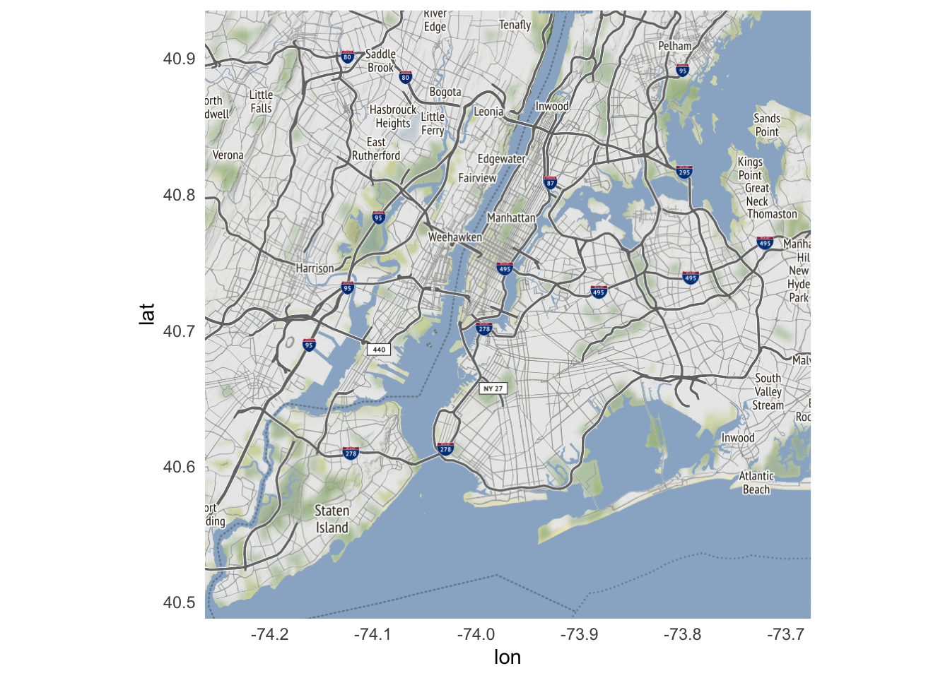
nyc_stamen <- get_stamenmap(
bbox = nyc_bb,
zoom = 11
)
nyc_stamen
## 859x854 terrain map image from Stamen Maps.
## See ?ggmap to plot it.
To view the map, use ggmap():
ggmap(nyc_stamen)
The zoom argument in get_stamenmap() controls the level of detail in the map. The larger the number, the greater the detail.
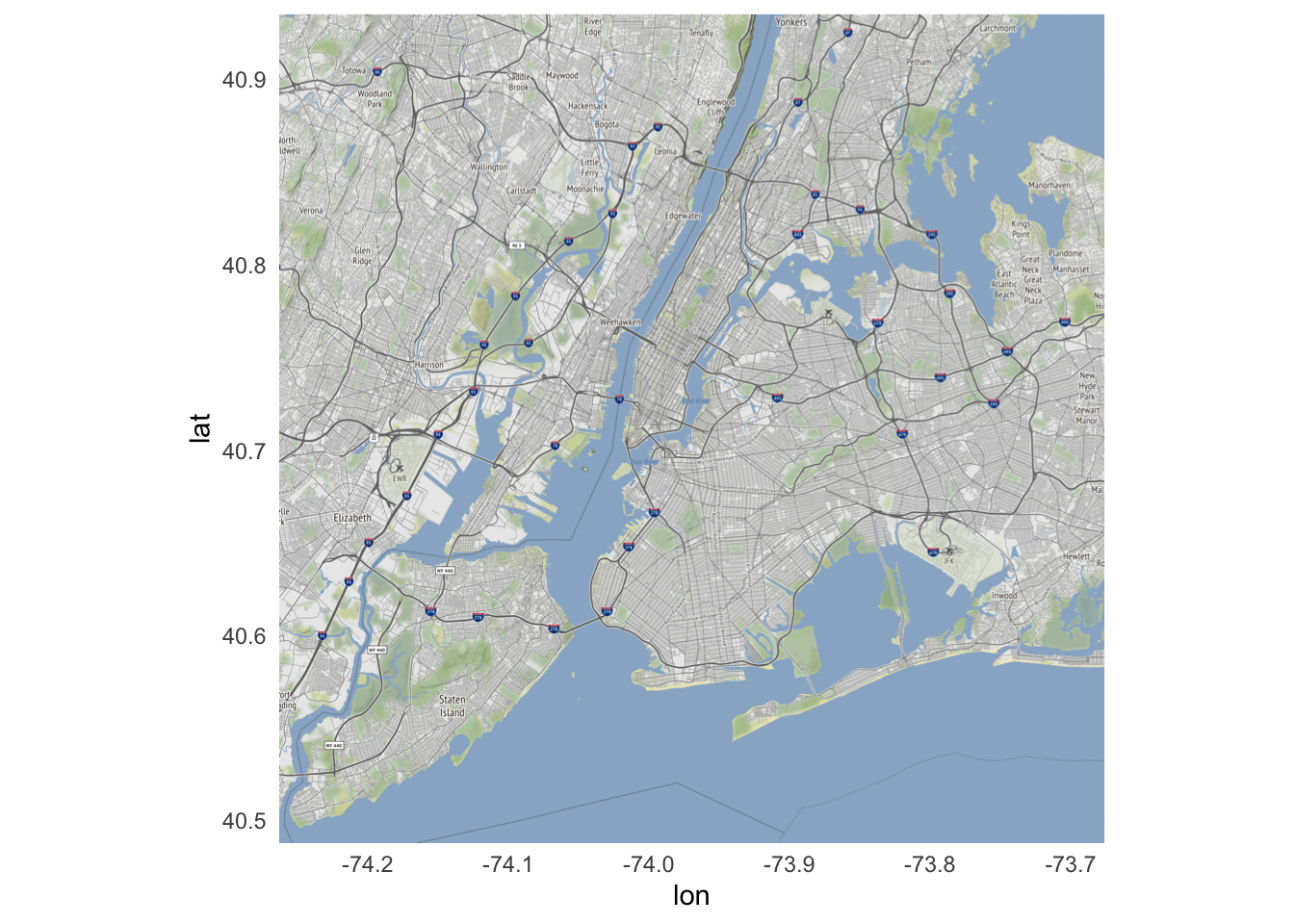
get_stamenmap(
  bbox = nyc_bb,
  zoom = 12
) %>%
  ggmap()
The smaller the number, the lesser the detail.
get_stamenmap(
  bbox = nyc_bb,
  zoom = 10
) %>%
  ggmap()
Trial and error will help you decide on the appropriate level of detail depending on what data you need to visualize on the map.
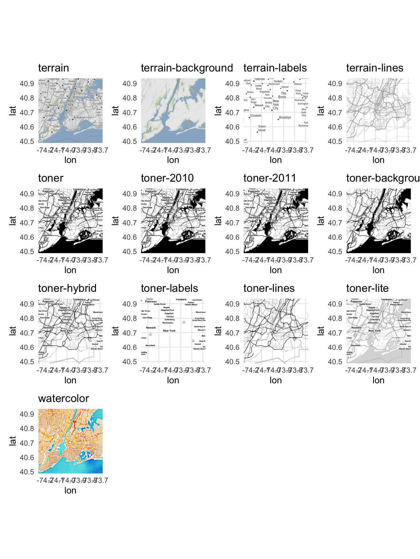
Types of map tiles
Each map tile provider offers a range of different types of maps depending on the background you want for the map. Stamen Maps offers several different types:
get_map() is a wrapper that automatically queries OpenStreetMap or Stamen Maps depending on the function arguments and inputs. While useful, it also combines all the different arguments of get_stamenmap() and getopenstreetmap() and can become a bit jumbled. Use at your own risk.Import crime data
Now that we can obtain map tiles and draw them using ggmap(), let’s explore how to add data to the map. New York City has an excellent data portal publishing a large volume of public records. Here we’ll look at crime data from 2022. I previously downloaded a .csv file containing all the records, which I import using read_csv():
crimes <- read_csv("https://info5940.infosci.cornell.edu/data/nyc-crimes.csv") to download the file from the course website.crimes <- here("static", "data", "nyc-crimes.csv") %>%
read_csv()
glimpse(crimes)
## Rows: 256,797
## Columns: 7
## $ cmplnt_num   <chr> "247350382", "243724728", "246348713", "240025455", "2461…
## $ boro_nm      <chr> "BROOKLYN", "QUEENS", "QUEENS", "BROOKLYN", "BRONX", "BRO…
## $ cmplnt_fr_dt <dttm> 1011-05-18 04:56:02, 1022-04-11 04:56:02, 1022-06-08 04:…
## $ law_cat_cd   <chr> "MISDEMEANOR", "MISDEMEANOR", "MISDEMEANOR", "FELONY", "F…
## $ ofns_desc    <chr> "CRIMINAL MISCHIEF & RELATED OF", "PETIT LARCENY", "PETIT…
## $ latitude     <dbl> 40.7, 40.8, 40.7, 40.7, 40.8, 40.7, 40.7, 40.7, 40.8, 40.…
## $ longitude    <dbl> -73.9, -73.8, -73.8, -74.0, -73.9, -74.0, -73.9, -73.9, -…
Each row of the data frame is a single reported incident of crime. Geographic location is encoded using the exact longitude and latitude of the incident.
Plot high-level map of crime
Let’s start with a simple high-level overview of reported crime in New York City. First we need a map for the entire city.
nyc <- nyc_stamen
ggmap(nyc)

Using geom_point()
Since each row is a single reported incident of crime, we could use geom_point() to map the location of every crime in the dataset. Because ggmap() uses the map tiles (here, defined by nyc) as the basic input, we specify data and mapping inside of geom_point(), rather than inside ggplot():
ggmap(nyc) +
  geom_point(
    data = crimes,
    mapping = aes(
      x = longitude,
      y = latitude
    )
  )
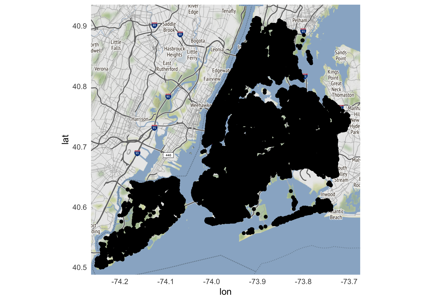
What went wrong? All we get is a sea of black.
nrow(crimes)
## [1] 256797
Oh yeah. There were 256,797 reported incidents of crime in the city. Each incident is represented by a dot on the map. How can we make this map more usable? One option is to decrease the size and increase the transparency of each data point so dense clusters of crime become apparent:
ggmap(nyc) +
  geom_point(
    data = crimes,
    aes(
      x = longitude,
      y = latitude
    ),
    size = .25,
    alpha = .01
  )
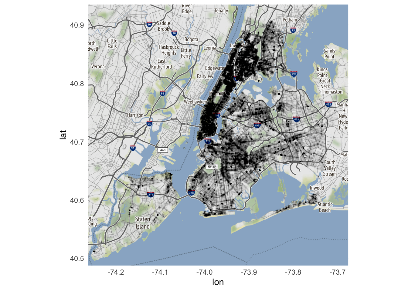
Better, but still not quite as useful as it could be.
Using stat_density_2d()
Instead of relying on geom_point() and plotting the raw data, a better approach is to create a heatmap. More precisely, this will be a two-dimensional kernel density estimation (KDE). In this context, KDE will take all the raw data (i.e. reported incidents of crime) and convert it into a smoothed plot showing geographic concentrations of crime. The core function in ggplot2 to generate this kind of plot is geom_density_2d():
ggmap(nyc) +
  geom_density_2d(
    data = crimes,
    aes(
      x = longitude,
      y = latitude
    )
  )
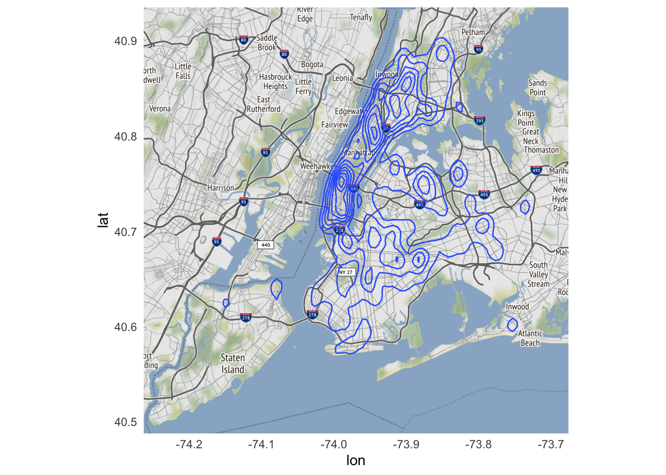
By default, geom_density_2d() draws a contour plot with lines of constant value. That is, each line represents approximately the same frequency of crime all along that specific line. Contour plots are frequently used in maps (known as topographic maps) to denote elevation.
](/media/contour-map_hua50b97a337ebf4f1ff2f376bc62271a6_306658_5c7db9d53ef3ad3cd21905cf4ee15aeb.webp)
Rather than drawing lines, instead we can fill in the graph so that we use the fill aesthetic to draw bands of crime density. To do that, we use the related function stat_density_2d():
ggmap(nyc) +
  stat_density_2d(
    data = crimes,
    aes(
      x = longitude,
      y = latitude,
      fill = stat(level)
    ),
    geom = "polygon"
  )
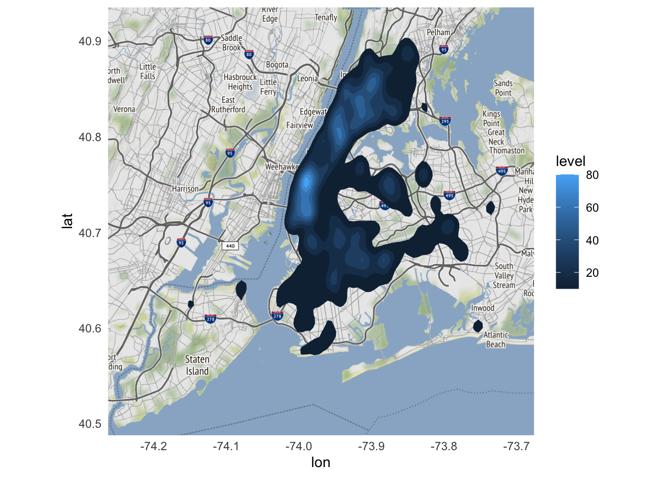
Note the two new arguments:
geom = "polygon"- change the geometric object to be drawn from adensity_2dgeom to apolygongeomfill = stat(level)- the value for thefillaesthetic is thelevelcalculated withinstat_density_2d(), which we access using thestat()notation.
This is an improvement, but we can adjust some additional settings to make the graph visually more useful. Specifically,
- Increase the number of
bins, or unique bands of color allowed on the graph - Make the heatmap semi-transparent using
alphaso we can still view the underlying map - Change the color palette to better distinguish between high and low crime areas. Here I use
brewer.pal()from theRColorBrewerpackage to create a custom color palette using reds and yellows.
ggmap(nyc) +
  stat_density_2d(
    data = crimes,
    aes(
      x = longitude,
      y = latitude,
      fill = stat(level)
    ),
    alpha = .2,
    bins = 25,
    geom = "polygon"
  ) +
  scale_fill_gradientn(colors = brewer.pal(7, "YlOrRd"))
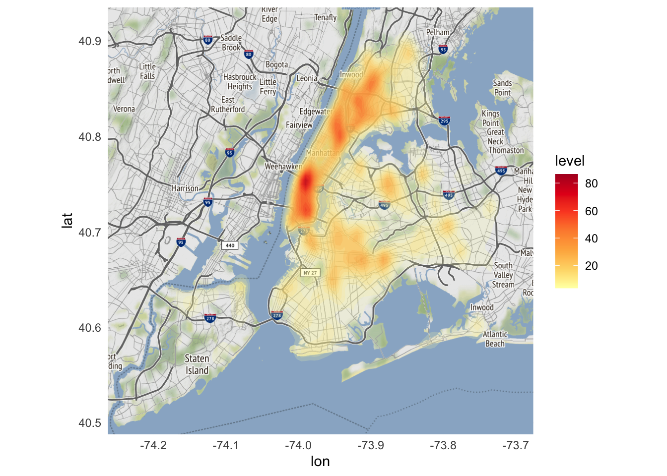
From this map, a couple trends are noticeable:
- The downtown region has the highest crime incidence rate. Not surprising given its population density during the workday.
- There are clusters of crime on the south and west sides. Also not surprising if you know anything about the city of Chicago.
Looking for variation
Because ggmap is built on ggplot2, we can use the core features of ggplot2 to modify the graph. One major feature is faceting. Let’s focus our analysis on four types of crimes with similar frequency of reported incidents1 and facet by type of crime:
ggmap(nyc) +
  stat_density_2d(
    data = crimes %>%
      filter(ofns_desc %in% c(
        "DANGEROUS DRUGS", "GRAND LARCENY OF MOTOR VEHICLE",
        "ROBBERY", "VEHICLE AND TRAFFIC LAWS"
      )),
    aes(
      x = longitude,
      y = latitude,
      fill = stat(level)
    ),
    alpha = .4,
    bins = 10,
    geom = "polygon"
  ) +
  scale_fill_gradientn(colors = brewer.pal(7, "YlOrRd")) +
  facet_wrap(facets = vars(ofns_desc))
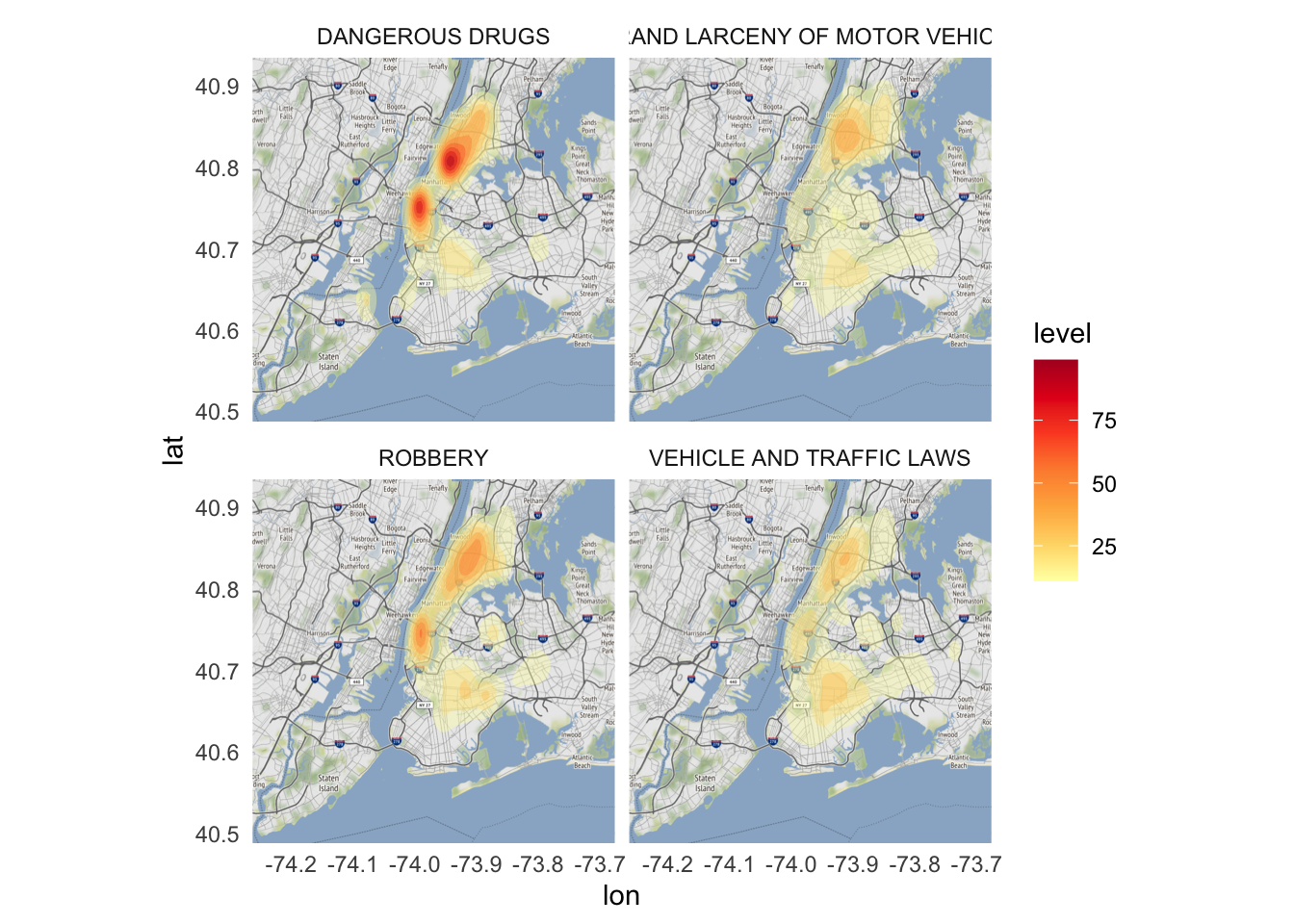
There is a substantial difference in the geographic density of drug crimes relative to the other categories. While burglaries, motor vehicle thefts, and robberies are reasonably prevalent all across the city, the vast majority of narcotics crimes occur in Manhattan and the Bronx.
Locations of murders
While geom_point() was not appropriate for graphing a large number of observations in a dense geographic location, it does work rather well for less dense areas. Now let’s limit our analysis strictly to reported incidents of murder.
(homicides <- crimes %>%
  filter(ofns_desc == "MURDER & NON-NEGL. MANSLAUGHTER"))
## # A tibble: 269 × 7
## cmplnt_num boro_nm cmplnt_fr_dt law_cat…¹ ofns_…² latit…³ longi…⁴
## <chr> <chr> <dttm> <chr> <chr> <dbl> <dbl>
## 1 240954923H1 BROOKLYN 1977-12-20 05:00:00 FELONY MURDER… 40.7 -74.0
## 2 245958045H1 BROOKLYN 2001-08-13 04:00:00 FELONY MURDER… 40.7 -73.9
## 3 8101169H6113 MANHATTAN 2005-03-06 05:00:00 FELONY MURDER… 40.8 -73.9
## 4 8101169H6113 MANHATTAN 2005-03-06 05:00:00 FELONY MURDER… 40.8 -73.9
## 5 16631466H8909 BROOKLYN 2006-05-24 04:00:00 FELONY MURDER… 40.7 -73.9
## 6 246056367H1 QUEENS 2015-05-13 04:00:00 FELONY MURDER… 40.6 -73.7
## 7 243507594H1 MANHATTAN 2020-06-19 04:00:00 FELONY MURDER… 40.8 -74.0
## 8 243688124H1 BROOKLYN 2021-01-31 05:00:00 FELONY MURDER… 40.7 -73.9
## 9 240767513H1 BROOKLYN 2021-02-17 05:00:00 FELONY MURDER… 40.6 -74.0
## 10 240767512H1 BROOKLYN 2021-05-24 04:00:00 FELONY MURDER… 40.6 -74.0
## # … with 259 more rows, and abbreviated variable names ¹law_cat_cd, ²ofns_desc,
## # ³latitude, ⁴longitude
We can draw a map of the city with all homicides indicated on the map using geom_point():
ggmap(nyc) +
  geom_point(
    data = homicides,
    mapping = aes(
      x = longitude,
      y = latitude
    ),
    size = 1
  )
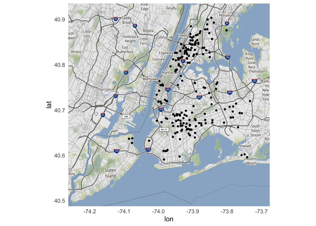
Compared to our previous overviews, few if any homicides are reported in downtown Manhattan.
We can also narrow down the geographic location to map specific neighborhoods in New York City. First we obtain map tiles for those ares. Here we’ll examine Roosevelt Island and Fordham.
# compare Roosevelt Island to Harlem
roosevelt_bb <- c(
  left = -73.993958,
  bottom = 40.737279,
  right = -73.912204,
  top = 40.780838
)
roosevelt <- get_stamenmap(
  bbox = roosevelt_bb,
  zoom = 14
)

fordham_bb <- c(
  left = -73.939754,
  bottom = 40.837444,
  right = -73.858000,
  top = 40.880937
)
fordham <- get_stamenmap(
  bbox = fordham_bb,
  zoom = 14
)

ggmap(roosevelt)
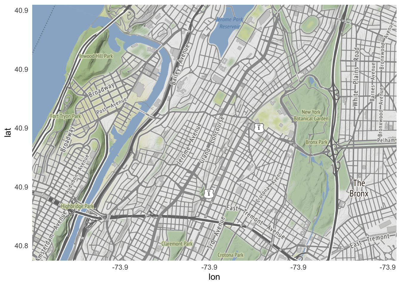
ggmap(fordham)
To plot homicides specifically in these neighborhoods, change ggmap(nyc) to the appropriate map tile:
ggmap(roosevelt) +
  geom_point(
    data = homicides,
    aes(x = longitude, y = latitude)
  )

ggmap(fordham) +
  geom_point(
    data = homicides,
    aes(x = longitude, y = latitude)
  )
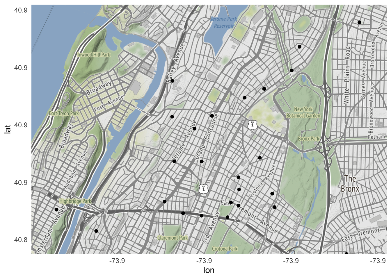
Even though homicides contained data for homicides across the entire city, ggmap() automatically cropped the graph to keep just the homicides that occurred within the bounding box.
All the other aesthetic customizations of geom_point() work with ggmap. So we could expand these neighborhood maps to include all violent crimes2 and distinguish each type by color:
(violent <- crimes %>%
  filter(ofns_desc %in% c(
    "MURDER & NON-NEGL. MANSLAUGHTER",
    "RAPE",
    "ROBBERY",
    "FELONY ASSAULT"
  )))
## # A tibble: 21,723 × 7
## cmplnt_num boro_nm cmplnt_fr_dt law_cat_cd ofns_d…¹ latit…² longi…³
## <chr> <chr> <dttm> <chr> <chr> <dbl> <dbl>
## 1 240954923H1 BROOKLYN 1977-12-20 05:00:00 FELONY MURDER … 40.7 -74.0
## 2 244898507 BROOKLYN 1983-07-01 04:00:00 FELONY RAPE 40.6 -74.0
## 3 245625141 QUEENS 1998-01-01 05:00:00 FELONY RAPE 40.7 -73.8
## 4 241761571 BRONX 2000-03-08 05:00:00 FELONY ROBBERY 40.8 -73.9
## 5 245183845 BROOKLYN 2000-05-16 04:00:00 FELONY RAPE 40.7 -74.0
## 6 241162822 QUEENS 2000-09-01 04:00:00 FELONY RAPE 40.7 -73.8
## 7 242903456 BRONX 2001-01-01 05:00:00 FELONY RAPE 40.8 -73.9
## 8 245958045H1 BROOKLYN 2001-08-13 04:00:00 FELONY MURDER … 40.7 -73.9
## 9 247319927 BRONX 2002-06-29 04:00:00 FELONY ROBBERY 40.9 -73.8
## 10 239503898 MANHATTAN 2002-12-01 05:00:00 FELONY RAPE 40.7 -74.0
## # … with 21,713 more rows, and abbreviated variable names ¹ofns_desc,
## # ²latitude, ³longitude
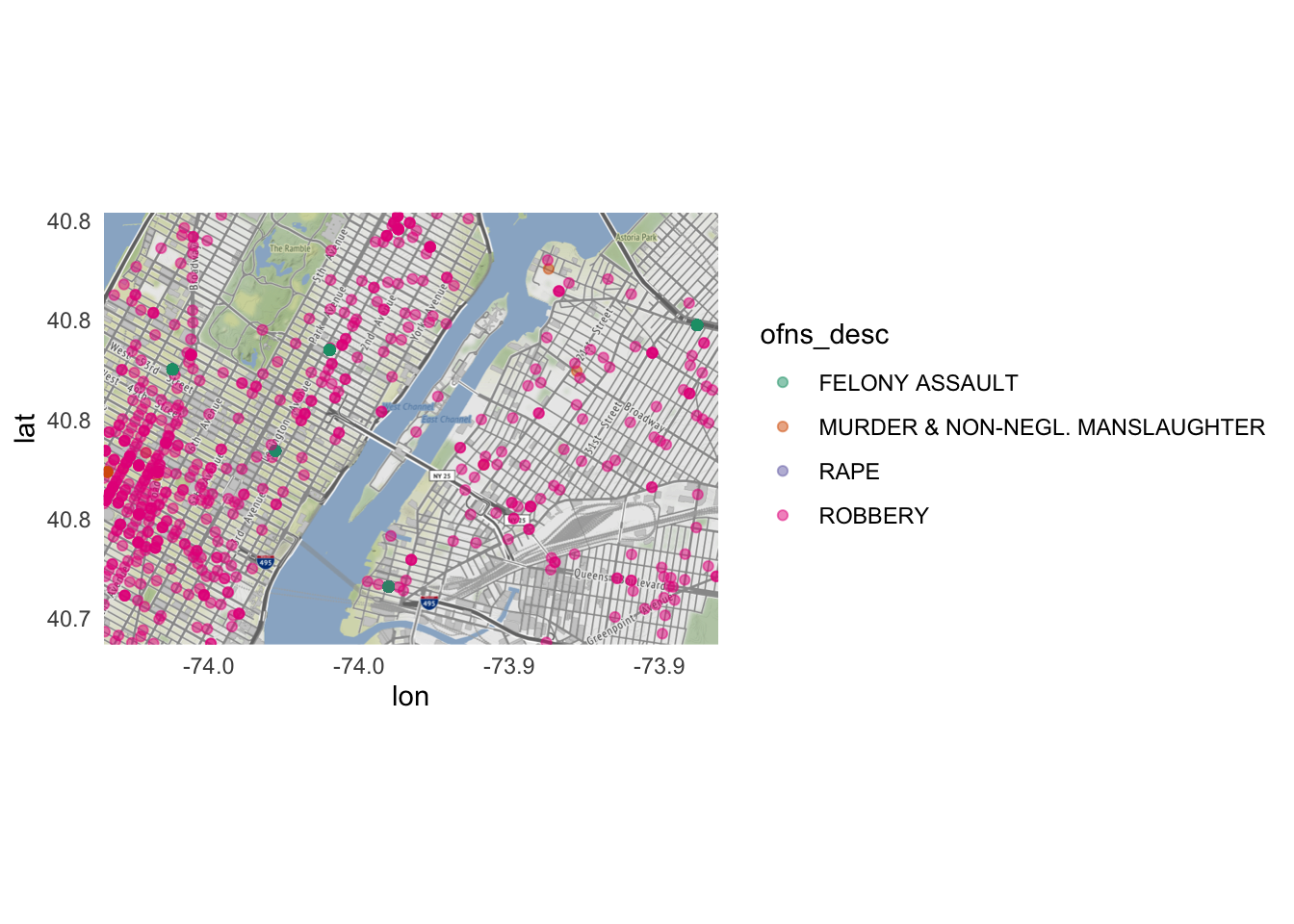
ggmap(roosevelt) +
  geom_point(
    data = violent,
    aes(
      x = longitude, y = latitude,
      color = ofns_desc
    ),
    alpha = 0.5
  ) +
  scale_color_brewer(type = "qual", palette = "Dark2")
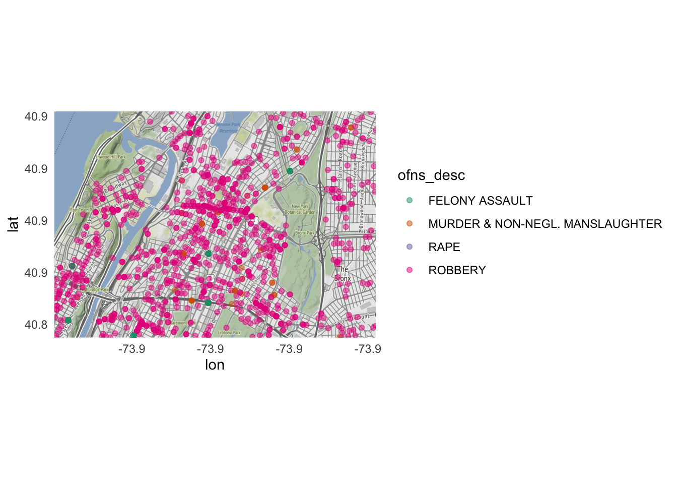
ggmap(fordham) +
  geom_point(
    data = violent,
    aes(
      x = longitude, y = latitude,
      color = ofns_desc
    ),
    alpha = 0.5
  ) +
  scale_color_brewer(type = "qual", palette = "Dark2")
Additional resources
Session Info
sessioninfo::session_info()
## ─ Session info ───────────────────────────────────────────────────────────────
##  setting  value
##  version  R version 4.2.1 (2022-06-23)
##  os       macOS Monterey 12.3
##  system   aarch64, darwin20
##  ui       X11
##  language (EN)
##  collate  en_US.UTF-8
##  ctype    en_US.UTF-8
##  tz       America/New_York
##  date     2022-10-05
##  pandoc   2.18 @ /Applications/RStudio.app/Contents/MacOS/quarto/bin/tools/ (via rmarkdown)
##
## ─ Packages ───────────────────────────────────────────────────────────────────
##  package       * version    date (UTC) lib source
##  assertthat      0.2.1      2019-03-21 [2] CRAN (R 4.2.0)
##  backports       1.4.1      2021-12-13 [2] CRAN (R 4.2.0)
##  bit             4.0.4      2020-08-04 [2] CRAN (R 4.2.0)
##  bit64           4.0.5      2020-08-30 [2] CRAN (R 4.2.0)
##  bitops          1.0-7      2021-04-24 [2] CRAN (R 4.2.0)
##  blogdown        1.10       2022-05-10 [2] CRAN (R 4.2.0)
##  bookdown        0.27       2022-06-14 [2] CRAN (R 4.2.0)
##  broom           1.0.0      2022-07-01 [2] CRAN (R 4.2.0)
##  bslib           0.4.0      2022-07-16 [2] CRAN (R 4.2.0)
##  cachem          1.0.6      2021-08-19 [2] CRAN (R 4.2.0)
##  cellranger      1.1.0      2016-07-27 [2] CRAN (R 4.2.0)
##  class           7.3-20     2022-01-16 [2] CRAN (R 4.2.1)
##  classInt        0.4-7      2022-06-10 [2] CRAN (R 4.2.0)
##  cli             3.4.0      2022-09-08 [1] CRAN (R 4.2.0)
##  codetools       0.2-18     2020-11-04 [2] CRAN (R 4.2.1)
##  colorspace      2.0-3      2022-02-21 [2] CRAN (R 4.2.0)
##  crayon          1.5.1      2022-03-26 [2] CRAN (R 4.2.0)
##  curl            4.3.2      2021-06-23 [2] CRAN (R 4.2.0)
##  DBI             1.1.3      2022-06-18 [2] CRAN (R 4.2.0)
##  dbplyr          2.2.1      2022-06-27 [2] CRAN (R 4.2.0)
##  digest          0.6.29     2021-12-01 [2] CRAN (R 4.2.0)
##  dplyr         * 1.0.9      2022-04-28 [2] CRAN (R 4.2.0)
##  e1071           1.7-11     2022-06-07 [2] CRAN (R 4.2.0)
##  ellipsis        0.3.2      2021-04-29 [2] CRAN (R 4.2.0)
##  evaluate        0.16       2022-08-09 [1] CRAN (R 4.2.1)
##  fansi           1.0.3      2022-03-24 [2] CRAN (R 4.2.0)
##  farver          2.1.1      2022-07-06 [2] CRAN (R 4.2.0)
##  fastmap         1.1.0      2021-01-25 [2] CRAN (R 4.2.0)
##  forcats       * 0.5.1      2021-01-27 [2] CRAN (R 4.2.0)
##  fs              1.5.2      2021-12-08 [2] CRAN (R 4.2.0)
##  gargle          1.2.0      2021-07-02 [2] CRAN (R 4.2.0)
##  generics        0.1.3      2022-07-05 [2] CRAN (R 4.2.0)
##  ggmap         * 3.0.0      2019-02-05 [2] CRAN (R 4.2.0)
##  ggplot2       * 3.3.6      2022-05-03 [2] CRAN (R 4.2.0)
##  glue            1.6.2      2022-02-24 [2] CRAN (R 4.2.0)
##  googledrive     2.0.0      2021-07-08 [2] CRAN (R 4.2.0)
##  googlesheets4   1.0.0      2021-07-21 [2] CRAN (R 4.2.0)
##  gtable          0.3.0      2019-03-25 [2] CRAN (R 4.2.0)
##  haven           2.5.0      2022-04-15 [2] CRAN (R 4.2.0)
##  here          * 1.0.1      2020-12-13 [2] CRAN (R 4.2.0)
##  highr           0.9        2021-04-16 [2] CRAN (R 4.2.0)
##  hms             1.1.1      2021-09-26 [2] CRAN (R 4.2.0)
##  htmltools       0.5.3      2022-07-18 [2] CRAN (R 4.2.0)
##  httr            1.4.3      2022-05-04 [2] CRAN (R 4.2.0)
##  isoband         0.2.5      2021-07-13 [2] CRAN (R 4.2.0)
##  jpeg            0.1-9      2021-07-24 [2] CRAN (R 4.2.0)
##  jquerylib       0.1.4      2021-04-26 [2] CRAN (R 4.2.0)
##  jsonlite        1.8.0      2022-02-22 [2] CRAN (R 4.2.0)
##  KernSmooth      2.23-20    2021-05-03 [2] CRAN (R 4.2.1)
##  knitr           1.40       2022-08-24 [1] CRAN (R 4.2.0)
##  labeling        0.4.2      2020-10-20 [2] CRAN (R 4.2.0)
##  lattice         0.20-45    2021-09-22 [2] CRAN (R 4.2.1)
##  lifecycle       1.0.2      2022-09-09 [1] CRAN (R 4.2.0)
##  lubridate       1.8.0      2021-10-07 [2] CRAN (R 4.2.0)
##  magrittr        2.0.3      2022-03-30 [2] CRAN (R 4.2.0)
##  MASS            7.3-58.1   2022-08-03 [2] CRAN (R 4.2.0)
##  modelr          0.1.8      2020-05-19 [2] CRAN (R 4.2.0)
##  munsell         0.5.0      2018-06-12 [2] CRAN (R 4.2.0)
##  patchwork     * 1.1.1      2020-12-17 [2] CRAN (R 4.2.0)
##  pillar          1.8.1      2022-08-19 [1] CRAN (R 4.2.0)
##  pkgconfig       2.0.3      2019-09-22 [2] CRAN (R 4.2.0)
##  plyr            1.8.7      2022-03-24 [2] CRAN (R 4.2.0)
##  png             0.1-7      2013-12-03 [2] CRAN (R 4.2.0)
##  proxy           0.4-27     2022-06-09 [2] CRAN (R 4.2.0)
##  purrr         * 0.3.4      2020-04-17 [2] CRAN (R 4.2.0)
##  R6              2.5.1      2021-08-19 [2] CRAN (R 4.2.0)
##  RColorBrewer  * 1.1-3      2022-04-03 [2] CRAN (R 4.2.0)
##  Rcpp            1.0.9      2022-07-08 [2] CRAN (R 4.2.0)
##  readr         * 2.1.2      2022-01-30 [2] CRAN (R 4.2.0)
##  readxl          1.4.0      2022-03-28 [2] CRAN (R 4.2.0)
##  reprex          2.0.1.9000 2022-08-10 [1] Github (tidyverse/reprex@6d3ad07)
##  RgoogleMaps     1.4.5.3    2020-02-12 [2] CRAN (R 4.2.0)
##  rjson           0.2.21     2022-01-09 [2] CRAN (R 4.2.0)
##  rlang           1.0.5      2022-08-31 [1] CRAN (R 4.2.0)
##  rmarkdown       2.14       2022-04-25 [2] CRAN (R 4.2.0)
##  rprojroot       2.0.3      2022-04-02 [2] CRAN (R 4.2.0)
##  rstudioapi      0.13       2020-11-12 [2] CRAN (R 4.2.0)
##  rvest           1.0.2      2021-10-16 [2] CRAN (R 4.2.0)
##  sass            0.4.2      2022-07-16 [2] CRAN (R 4.2.0)
##  scales          1.2.0      2022-04-13 [2] CRAN (R 4.2.0)
##  sessioninfo     1.2.2      2021-12-06 [2] CRAN (R 4.2.0)
##  sf            * 1.0-8      2022-07-14 [2] CRAN (R 4.2.0)
##  sp              1.5-0      2022-06-05 [2] CRAN (R 4.2.0)
##  stringi         1.7.8      2022-07-11 [2] CRAN (R 4.2.0)
##  stringr       * 1.4.0      2019-02-10 [2] CRAN (R 4.2.0)
##  tibble        * 3.1.8      2022-07-22 [2] CRAN (R 4.2.0)
##  tidyr         * 1.2.0      2022-02-01 [2] CRAN (R 4.2.0)
##  tidyselect      1.1.2      2022-02-21 [2] CRAN (R 4.2.0)
##  tidyverse     * 1.3.2      2022-07-18 [2] CRAN (R 4.2.0)
##  tzdb            0.3.0      2022-03-28 [2] CRAN (R 4.2.0)
##  units           0.8-0      2022-02-05 [2] CRAN (R 4.2.0)
##  utf8            1.2.2      2021-07-24 [2] CRAN (R 4.2.0)
##  vctrs           0.4.1      2022-04-13 [2] CRAN (R 4.2.0)
##  vroom           1.5.7      2021-11-30 [2] CRAN (R 4.2.0)
##  withr           2.5.0      2022-03-03 [2] CRAN (R 4.2.0)
##  xfun            0.31       2022-05-10 [1] CRAN (R 4.2.0)
##  xml2            1.3.3      2021-11-30 [2] CRAN (R 4.2.0)
##  yaml            2.3.5      2022-02-21 [2] CRAN (R 4.2.0)
##
##  [1] /Users/soltoffbc/Library/R/arm64/4.2/library
##  [2] /Library/Frameworks/R.framework/Versions/4.2-arm64/Resources/library
##
## ──────────────────────────────────────────────────────────────────────────────
Specifically drugs, motor vehicle thefts, robbery, and other vehicle/traffic crimes. ↩︎
The FBI defines violent crime as one of four offenses: murder and nonnegligent manslaughter, forcible rape, robbery, and aggravated assault. In the NYPD database, the comparable categories are murder and nonnegligent manslaughter, rape, robbery, and felony assault. ↩︎