Practice exploring college education (data)
library(tidyverse)
Run the code below in your console to download this exercise as a set of R scripts.
usethis::use_course("cis-ds/exploratory-data-analysis")
The Department of Education collects annual statistics on colleges and universities in the United States. I have included a subset of this data from 2018-19 in the rcis library from GitHub. To install the package, run the command remotes::install_github("cis-ds/rcis") in the console.
remotes library installed, you will get an error. Go back and install this first using install.packages("remotes"), then run remotes::install_github("cis-ds/rcis").library(rcis)
data("scorecard")
glimpse(scorecard)
## Rows: 1,732
## Columns: 14
## $ unitid    <dbl> 100654, 100663, 100706, 100724, 100751, 100830, 100858, 1009…
## $ name      <chr> "Alabama A & M University", "University of Alabama at Birmin…
## $ state     <chr> "AL", "AL", "AL", "AL", "AL", "AL", "AL", "AL", "AL", "AL", …
## $ type      <fct> "Public", "Public", "Public", "Public", "Public", "Public", …
## $ admrate   <dbl> 0.9175, 0.7366, 0.8257, 0.9690, 0.8268, 0.9044, 0.8067, 0.53…
## $ satavg    <dbl> 939, 1234, 1319, 946, 1261, 1082, 1300, 1230, 1066, NA, 1076…
## $ cost      <dbl> 23053, 24495, 23917, 21866, 29872, 19849, 31590, 32095, 3431…
## $ netcost   <dbl> 14990, 16953, 15860, 13650, 22597, 13987, 24104, 22107, 2071…
## $ avgfacsal <dbl> 69381, 99441, 87192, 64989, 92619, 71343, 96642, 56646, 5400…
## $ pctpell   <dbl> 0.7019, 0.3512, 0.2536, 0.7627, 0.1772, 0.4644, 0.1455, 0.23…
## $ comprate  <dbl> 0.2974, 0.6340, 0.5768, 0.3276, 0.7110, 0.3401, 0.7911, 0.69…
## $ firstgen  <dbl> 0.3658281, 0.3412237, 0.3101322, 0.3434343, 0.2257127, 0.381…
## $ debt      <dbl> 15250, 15085, 14000, 17500, 17671, 12000, 17500, 16000, 1425…
## $ locale    <fct> City, City, City, City, City, City, City, City, City, Suburb…
Type ?scorecard in the console to open up the help file for this data set. This includes the documentation for all the variables. Use your knowledge of dplyr and ggplot2 functions to answer the following questions.
Which type of college has the highest average SAT score?
NOTE: This time, use a graph to visualize your answer, not a table.
Click for the solution
We could use a boxplot to visualize the distribution of SAT scores.
ggplot(
  data = scorecard,
  mapping = aes(x = type, y = satavg)
) +
  geom_boxplot()
## Warning: Removed 473 rows containing non-finite values (stat_boxplot).
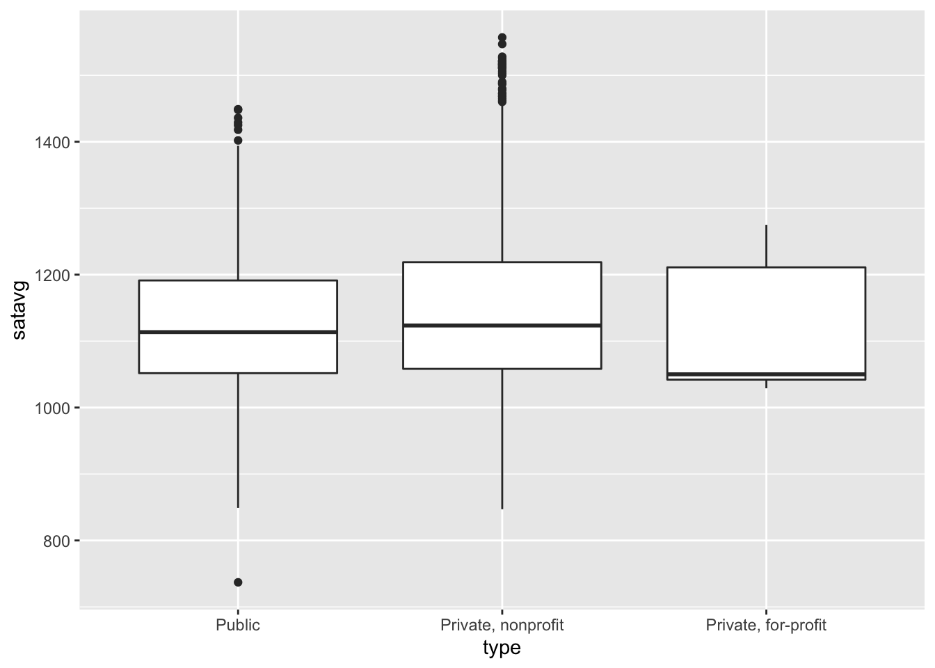
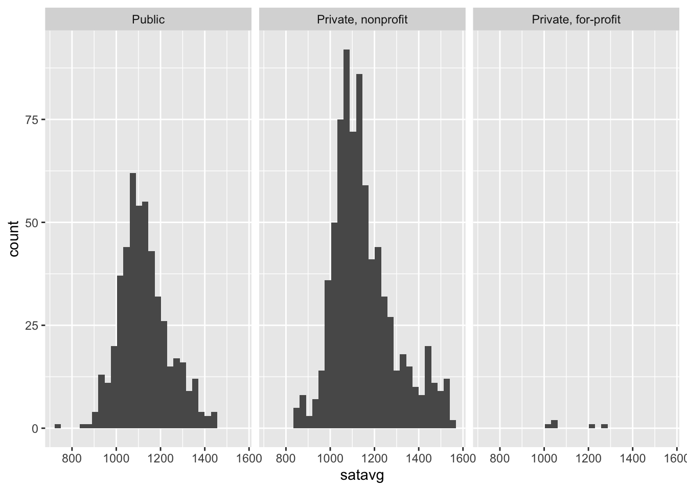
According to this graph, private, nonprofit schools have the highest average SAT score, followed by public and then private, for-profit schools. But this doesn’t reveal the entire picture. What happens if we plot a histogram or frequency polygon?
ggplot(
  data = scorecard,
  mapping = aes(x = satavg)
) +
  geom_histogram() +
  facet_wrap(facets = vars(type))
## `stat_bin()` using `bins = 30`. Pick better value with `binwidth`.
## Warning: Removed 473 rows containing non-finite values (stat_bin).
ggplot(
  data = scorecard,
  mapping = aes(x = satavg, color = type)
) +
  geom_freqpoly()
## `stat_bin()` using `bins = 30`. Pick better value with `binwidth`.
## Warning: Removed 473 rows containing non-finite values (stat_bin).
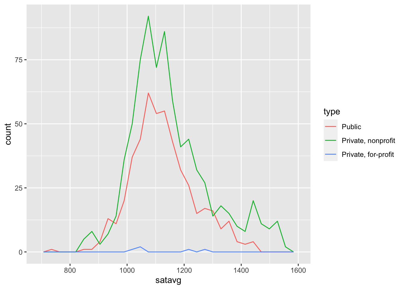
Now we can see the averages for each college type are based on widely varying sample sizes.
# observations with non-NA SAT averages
scorecard %>%
  drop_na(satavg) %>%
  ggplot(
    mapping = aes(x = type)
  ) +
  geom_bar()
# what proportion of observations have NA for satavg?
scorecard %>%
  group_by(type) %>%
  summarize(prop = sum(is.na(satavg)) / n()) %>%
  ggplot(
    mapping = aes(x = type, y = prop)
  ) +
  geom_col()
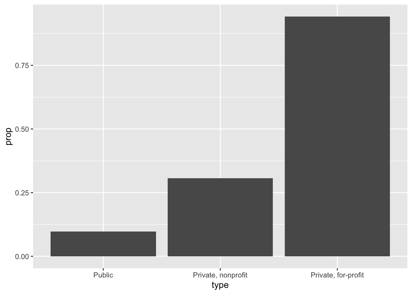
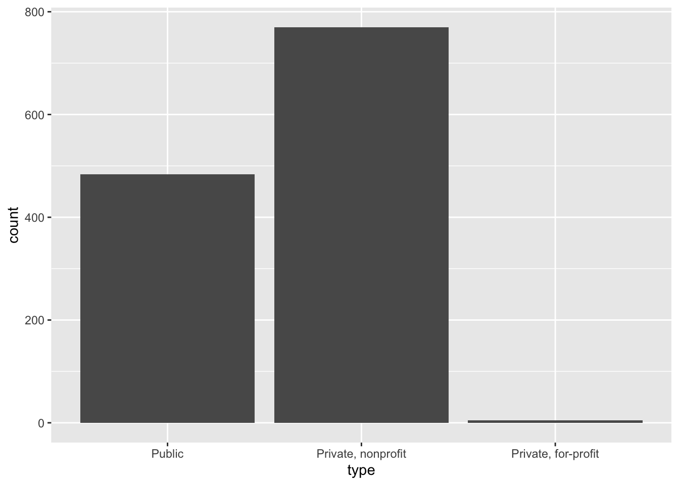
There are far fewer private, for-profit colleges than the other categories. Furthermore, private, for-profit colleges disproportionately fail to report average SAT scores compared to the other categories (likely these schools do not require SAT scores from applicants). A boxplot alone would not reveal this detail, which could be important in future analysis.
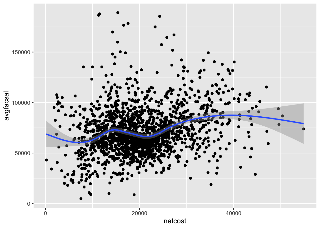
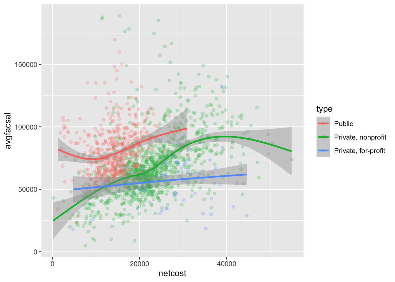
What is the relationship between net cost of attendance and faculty salaries? How does this relationship differ across types of colleges?
Click for the solution
# geom_point
ggplot(
  data = scorecard,
  mapping = aes(x = netcost, y = avgfacsal)
) +
  geom_point() +
  geom_smooth()
## `geom_smooth()` using method = 'gam' and formula 'y ~ s(x, bs = "cs")'
## Warning: Removed 55 rows containing non-finite values (stat_smooth).
## Warning: Removed 55 rows containing missing values (geom_point).
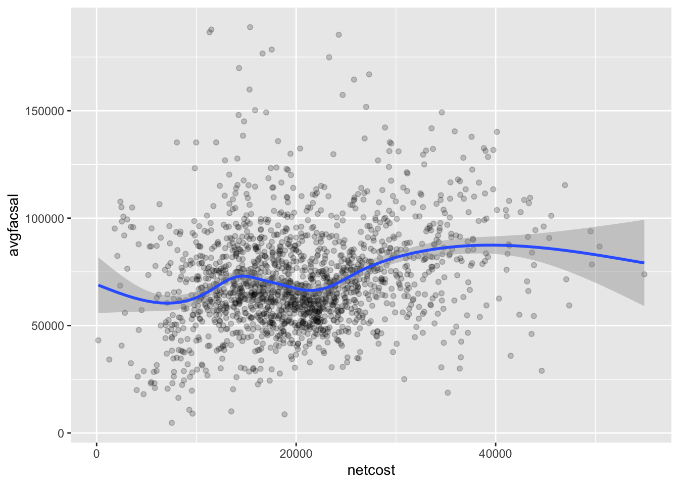
# geom_point with alpha transparency to reveal dense clusters
ggplot(
  data = scorecard,
  mapping = aes(x = netcost, y = avgfacsal)
) +
  geom_point(alpha = .2) +
  geom_smooth()
## `geom_smooth()` using method = 'gam' and formula 'y ~ s(x, bs = "cs")'
## Warning: Removed 55 rows containing non-finite values (stat_smooth).
## Removed 55 rows containing missing values (geom_point).
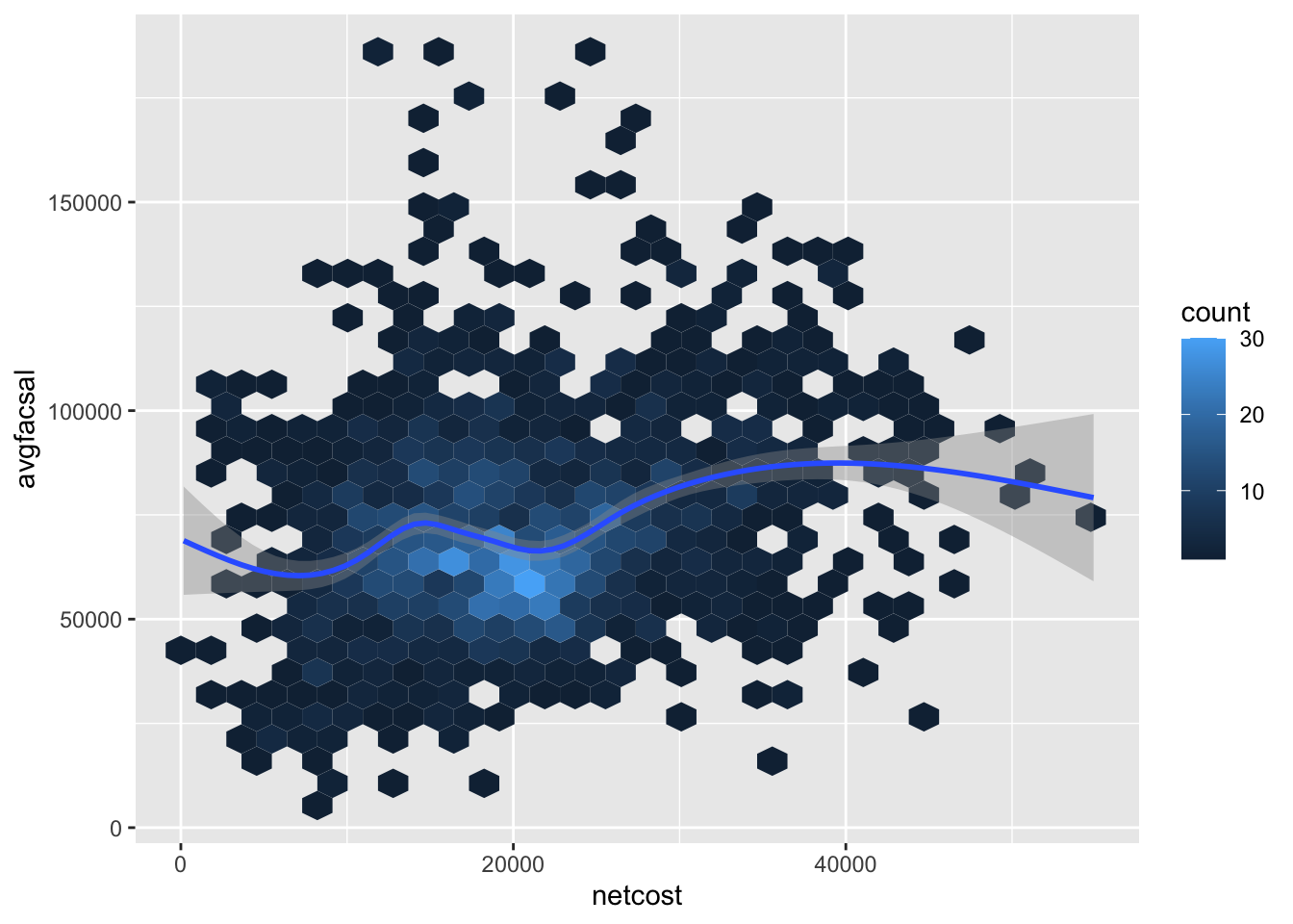
# geom_hex
ggplot(
  data = scorecard,
  mapping = aes(x = netcost, y = avgfacsal)
) +
  geom_hex() +
  geom_smooth()
## Warning: Removed 55 rows containing non-finite values (stat_binhex).
## `geom_smooth()` using method = 'gam' and formula 'y ~ s(x, bs = "cs")'
## Warning: Removed 55 rows containing non-finite values (stat_smooth).
# geom_point with smoothing lines for each type
ggplot(
  data = scorecard,
  mapping = aes(
    x = netcost,
    y = avgfacsal,
    color = type
  )
) +
  geom_point(alpha = .2) +
  geom_smooth()
## `geom_smooth()` using method = 'gam' and formula 'y ~ s(x, bs = "cs")'
## Warning: Removed 55 rows containing non-finite values (stat_smooth).
## Removed 55 rows containing missing values (geom_point).
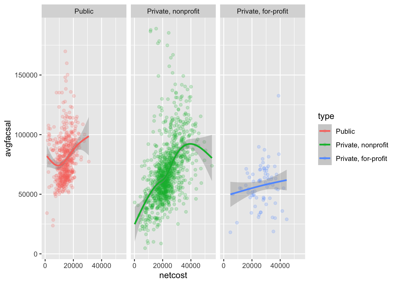
# geom_point with facets for each type
ggplot(
  data = scorecard,
  mapping = aes(
    x = netcost,
    y = avgfacsal,
    color = type
  )
) +
  geom_point(alpha = .2) +
  geom_smooth() +
  facet_grid(cols = vars(type))
## `geom_smooth()` using method = 'gam' and formula 'y ~ s(x, bs = "cs")'
## Warning: Removed 55 rows containing non-finite values (stat_smooth).
## Removed 55 rows containing missing values (geom_point).
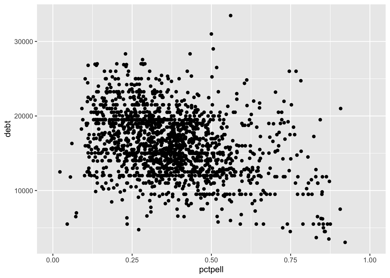
How are a college’s Pell Grant recipients related to the average student’s education debt?
Click for the solution
Two continuous variables suggest a scatterplot would be appropriate.
ggplot(
  data = scorecard,
  mapping = aes(x = pctpell, y = debt)
) +
  geom_point()
## Warning: Removed 112 rows containing missing values (geom_point).

Hmm. There seem to be a lot of data points. It isn’t really clear if there is a trend. What if we jitter the data points?
ggplot(
  data = scorecard,
  mapping = aes(x = pctpell, y = debt)
) +
  geom_jitter()
## Warning: Removed 112 rows containing missing values (geom_point).
Meh, didn’t really do much. What if we make our data points semi-transparent using the alpha aesthetic?
ggplot(
  data = scorecard,
  mapping = aes(x = pctpell, y = debt)
) +
  geom_point(alpha = .2)
## Warning: Removed 112 rows containing missing values (geom_point).
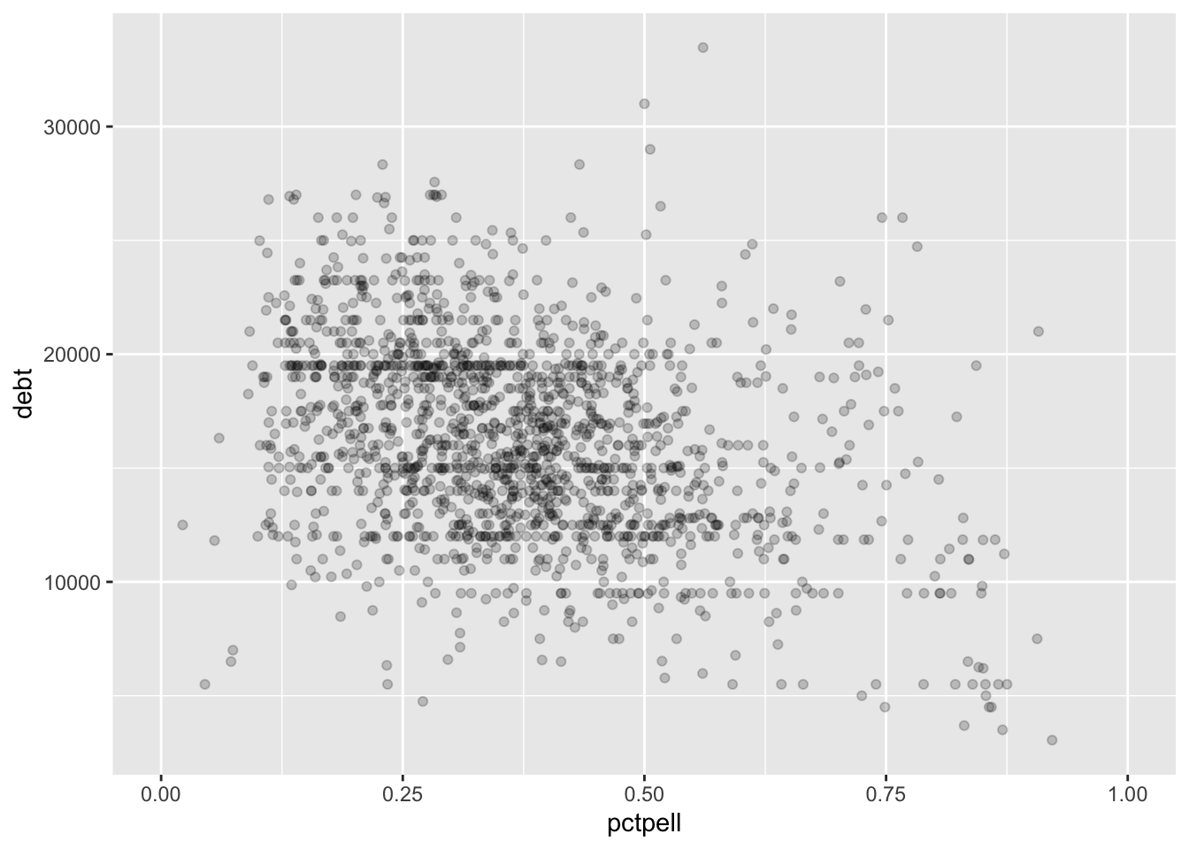
Now we’re getting somewhere. I’m beginning to see some dense clusters in the middle. Maybe a hexagon binning plot would help
ggplot(
  data = scorecard,
  mapping = aes(x = pctpell, y = debt)
) +
  geom_hex()
## Warning: Removed 112 rows containing non-finite values (stat_binhex).
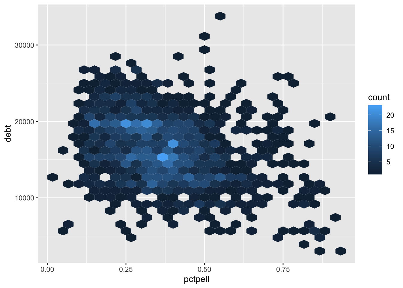
This is getting better. It looks like there might be a downward trend; that is, as the percentage of Pell grant recipients increases, average student debt decreases. Let’s confirm this by going back to the scatterplot and overlaying a smoothing line.
ggplot(
  data = scorecard,
  mapping = aes(x = pctpell, y = debt)
) +
  geom_point(alpha = .2) +
  geom_smooth()
## `geom_smooth()` using method = 'gam' and formula 'y ~ s(x, bs = "cs")'
## Warning: Removed 112 rows containing non-finite values (stat_smooth).
## Warning: Removed 112 rows containing missing values (geom_point).
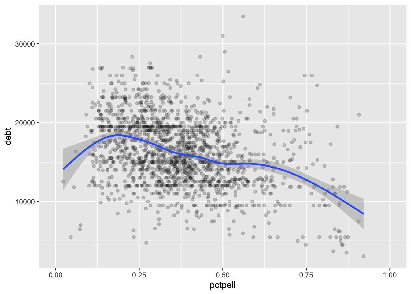
This confirms our initial evidence - there is an apparent negative relationship. Notice how I iterated through several different plots before I created one that provided the most informative visualization. You will not create the perfect graph on your first attempt. Trial and error is necessary in this exploratory stage. Be prepared to revise your code again and again.
Session Info
sessioninfo::session_info()
## ─ Session info ───────────────────────────────────────────────────────────────
##  setting  value
##  version  R version 4.2.1 (2022-06-23)
##  os       macOS Monterey 12.3
##  system   aarch64, darwin20
##  ui       X11
##  language (EN)
##  collate  en_US.UTF-8
##  ctype    en_US.UTF-8
##  tz       America/New_York
##  date     2022-10-05
##  pandoc   2.18 @ /Applications/RStudio.app/Contents/MacOS/quarto/bin/tools/ (via rmarkdown)
##
## ─ Packages ───────────────────────────────────────────────────────────────────
##  package       * version    date (UTC) lib source
##  assertthat      0.2.1      2019-03-21 [2] CRAN (R 4.2.0)
##  backports       1.4.1      2021-12-13 [2] CRAN (R 4.2.0)
##  blogdown        1.10       2022-05-10 [2] CRAN (R 4.2.0)
##  bookdown        0.27       2022-06-14 [2] CRAN (R 4.2.0)
##  broom           1.0.0      2022-07-01 [2] CRAN (R 4.2.0)
##  bslib           0.4.0      2022-07-16 [2] CRAN (R 4.2.0)
##  cachem          1.0.6      2021-08-19 [2] CRAN (R 4.2.0)
##  cellranger      1.1.0      2016-07-27 [2] CRAN (R 4.2.0)
##  cli             3.4.0      2022-09-08 [1] CRAN (R 4.2.0)
##  codetools       0.2-18     2020-11-04 [2] CRAN (R 4.2.1)
##  colorspace      2.0-3      2022-02-21 [2] CRAN (R 4.2.0)
##  crayon          1.5.1      2022-03-26 [2] CRAN (R 4.2.0)
##  DBI             1.1.3      2022-06-18 [2] CRAN (R 4.2.0)
##  dbplyr          2.2.1      2022-06-27 [2] CRAN (R 4.2.0)
##  digest          0.6.29     2021-12-01 [2] CRAN (R 4.2.0)
##  dplyr         * 1.0.9      2022-04-28 [2] CRAN (R 4.2.0)
##  ellipsis        0.3.2      2021-04-29 [2] CRAN (R 4.2.0)
##  evaluate        0.16       2022-08-09 [1] CRAN (R 4.2.1)
##  fansi           1.0.3      2022-03-24 [2] CRAN (R 4.2.0)
##  farver          2.1.1      2022-07-06 [2] CRAN (R 4.2.0)
##  fastmap         1.1.0      2021-01-25 [2] CRAN (R 4.2.0)
##  forcats       * 0.5.1      2021-01-27 [2] CRAN (R 4.2.0)
##  fs              1.5.2      2021-12-08 [2] CRAN (R 4.2.0)
##  gargle          1.2.0      2021-07-02 [2] CRAN (R 4.2.0)
##  generics        0.1.3      2022-07-05 [2] CRAN (R 4.2.0)
##  ggplot2       * 3.3.6      2022-05-03 [2] CRAN (R 4.2.0)
##  glue            1.6.2      2022-02-24 [2] CRAN (R 4.2.0)
##  googledrive     2.0.0      2021-07-08 [2] CRAN (R 4.2.0)
##  googlesheets4   1.0.0      2021-07-21 [2] CRAN (R 4.2.0)
##  gtable          0.3.0      2019-03-25 [2] CRAN (R 4.2.0)
##  haven           2.5.0      2022-04-15 [2] CRAN (R 4.2.0)
##  here            1.0.1      2020-12-13 [2] CRAN (R 4.2.0)
##  hexbin          1.28.2     2021-01-08 [2] CRAN (R 4.2.0)
##  highr           0.9        2021-04-16 [2] CRAN (R 4.2.0)
##  hms             1.1.1      2021-09-26 [2] CRAN (R 4.2.0)
##  htmltools       0.5.3      2022-07-18 [2] CRAN (R 4.2.0)
##  httr            1.4.3      2022-05-04 [2] CRAN (R 4.2.0)
##  jquerylib       0.1.4      2021-04-26 [2] CRAN (R 4.2.0)
##  jsonlite        1.8.0      2022-02-22 [2] CRAN (R 4.2.0)
##  knitr           1.40       2022-08-24 [1] CRAN (R 4.2.0)
##  labeling        0.4.2      2020-10-20 [2] CRAN (R 4.2.0)
##  lattice         0.20-45    2021-09-22 [2] CRAN (R 4.2.1)
##  lifecycle       1.0.2      2022-09-09 [1] CRAN (R 4.2.0)
##  lubridate       1.8.0      2021-10-07 [2] CRAN (R 4.2.0)
##  magrittr        2.0.3      2022-03-30 [2] CRAN (R 4.2.0)
##  Matrix          1.4-1      2022-03-23 [2] CRAN (R 4.2.1)
##  mgcv            1.8-40     2022-03-29 [2] CRAN (R 4.2.1)
##  modelr          0.1.8      2020-05-19 [2] CRAN (R 4.2.0)
##  munsell         0.5.0      2018-06-12 [2] CRAN (R 4.2.0)
##  nlme            3.1-158    2022-06-15 [2] CRAN (R 4.2.0)
##  pillar          1.8.1      2022-08-19 [1] CRAN (R 4.2.0)
##  pkgconfig       2.0.3      2019-09-22 [2] CRAN (R 4.2.0)
##  purrr         * 0.3.4      2020-04-17 [2] CRAN (R 4.2.0)
##  R6              2.5.1      2021-08-19 [2] CRAN (R 4.2.0)
##  rcis          * 0.2.5      2022-08-08 [2] local
##  readr         * 2.1.2      2022-01-30 [2] CRAN (R 4.2.0)
##  readxl          1.4.0      2022-03-28 [2] CRAN (R 4.2.0)
##  reprex          2.0.1.9000 2022-08-10 [1] Github (tidyverse/reprex@6d3ad07)
##  rlang           1.0.5      2022-08-31 [1] CRAN (R 4.2.0)
##  rmarkdown       2.14       2022-04-25 [2] CRAN (R 4.2.0)
##  rprojroot       2.0.3      2022-04-02 [2] CRAN (R 4.2.0)
##  rstudioapi      0.13       2020-11-12 [2] CRAN (R 4.2.0)
##  rvest           1.0.2      2021-10-16 [2] CRAN (R 4.2.0)
##  sass            0.4.2      2022-07-16 [2] CRAN (R 4.2.0)
##  scales          1.2.0      2022-04-13 [2] CRAN (R 4.2.0)
##  sessioninfo     1.2.2      2021-12-06 [2] CRAN (R 4.2.0)
##  stringi         1.7.8      2022-07-11 [2] CRAN (R 4.2.0)
##  stringr       * 1.4.0      2019-02-10 [2] CRAN (R 4.2.0)
##  tibble        * 3.1.8      2022-07-22 [2] CRAN (R 4.2.0)
##  tidyr         * 1.2.0      2022-02-01 [2] CRAN (R 4.2.0)
##  tidyselect      1.1.2      2022-02-21 [2] CRAN (R 4.2.0)
##  tidyverse     * 1.3.2      2022-07-18 [2] CRAN (R 4.2.0)
##  tzdb            0.3.0      2022-03-28 [2] CRAN (R 4.2.0)
##  utf8            1.2.2      2021-07-24 [2] CRAN (R 4.2.0)
##  vctrs           0.4.1      2022-04-13 [2] CRAN (R 4.2.0)
##  withr           2.5.0      2022-03-03 [2] CRAN (R 4.2.0)
##  xfun            0.31       2022-05-10 [1] CRAN (R 4.2.0)
##  xml2            1.3.3      2021-11-30 [2] CRAN (R 4.2.0)
##  yaml            2.3.5      2022-02-21 [2] CRAN (R 4.2.0)
##
##  [1] /Users/soltoffbc/Library/R/arm64/4.2/library
##  [2] /Library/Frameworks/R.framework/Versions/4.2-arm64/Resources/library
##
## ──────────────────────────────────────────────────────────────────────────────