Tidy data

library(tidyverse)

Most data analysts and statisticians analyze data in a spreadsheet or tabular format. This is not the only way to store information,¹ however in the social sciences it has been the paradigm for many decades. Tidy data is a specific way of organizing data into a consistent format which plugs into the tidyverse set of packages for R. It is not the only way to store data and there are reasons why you might not store data in this format, but eventually you will probably need to convert your data to a tidy format in order to efficiently analyze it.

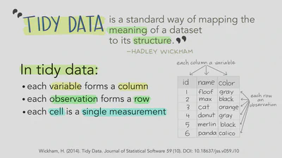
There are three rules which make a dataset tidy:

Each variable must have its own column.
Each observation must have its own row.
Each value must have its own cell.

Figure 12.1 from [*R for Data Science*](http://r4ds.had.co.nz) — Figure 12.1 from *R for Data Science*

Pivoting in `tidyr`

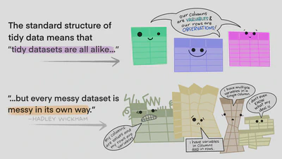
Most data you encounter in the wild is stored in an untidy format. To tidy the data, the basic approach is:

Identify what the observations and variables are
Fix the dataset so the observations are in rows and variables are in columns. Typically there is one of two problems in the data.
1. One variable might be spread across multiple columns.
2. One observation may be scattered across multiple rows.

Let’s review the different tasks for tidying data using the R for Data Science gapminder subset. This is the data in a tidy format:

table1

## # A tibble: 6 × 4
##   country      year  cases population
##   <chr>       <int>  <int>      <int>
## 1 Afghanistan  1999    745   19987071
## 2 Afghanistan  2000   2666   20595360
## 3 Brazil       1999  37737  172006362
## 4 Brazil       2000  80488  174504898
## 5 China        1999 212258 1272915272
## 6 China        2000 213766 1280428583

Note that in this data frame, each variable is in its own column (country, year, cases, and population), each observation is in its own row (i.e. each row is a different country-year pairing), and each value has its own cell.

Longer

tidyr contains two major functions that can be used to tidy datasets. pivot_longer() makes datasets longer by increasing the number of rows and decreasing the number of columns. Many datasets you obtain are optimized for ease of data entry or ease of comparison rather than ease of analysis. This means data is typically stored messy with more columns than necessary.

For example, this version of table1 is not tidy because the year variable is spread across multiple columns:

table4a

## # A tibble: 3 × 3
##   country     `1999` `2000`
## * <chr>        <int>  <int>
## 1 Afghanistan    745   2666
## 2 Brazil       37737  80488
## 3 China       212258 213766

To fix the data frame, we need to identify:

The set of columns whose names are values, not variables. Here, those are 1999 and 2000.
The name of the variable to move the column names to. Here it is year.
The name of the variable to move the column values to. Here it is cases.

We can use pivot_longer() to perform this operation:

table4a %>%
  pivot_longer(cols = c(`1999`, `2000`), names_to = "year", values_to = "cases")

## # A tibble: 6 × 3
##   country     year   cases
##   <chr>       <chr>  <int>
## 1 Afghanistan 1999     745
## 2 Afghanistan 2000    2666
## 3 Brazil      1999   37737
## 4 Brazil      2000   80488
## 5 China       1999  212258
## 6 China       2000  213766

Since 1999 and 2000 are non-standard names for columns (i.e. they start with a number), we have to wrap the column names in backticks.² Because year and cases don’t exist in table4a, we write them as character strings inside of quotation marks.

Wider

pivot_wider() is the opposite of pivot_longer(): it makes a dataset wider by increasing the number of columns and decreasing the number of rows. For instance, take table2:

table2

## # A tibble: 12 × 4
##    country      year type            count
##    <chr>       <int> <chr>           <int>
##  1 Afghanistan  1999 cases             745
##  2 Afghanistan  1999 population   19987071
##  3 Afghanistan  2000 cases            2666
##  4 Afghanistan  2000 population   20595360
##  5 Brazil       1999 cases           37737
##  6 Brazil       1999 population  172006362
##  7 Brazil       2000 cases           80488
##  8 Brazil       2000 population  174504898
##  9 China        1999 cases          212258
## 10 China        1999 population 1272915272
## 11 China        2000 cases          213766
## 12 China        2000 population 1280428583

It violates the tidy data principle because each observation (unit of analysis is a country-year pairing) is split across multiple rows. To tidy the data frame, we need to know:

The column that contains variable names. Here, it is type.
The column that contains values for multiple variables. Here it is count.

We can then use pivot_wider():

table2 %>%
  pivot_wider(names_from = type, values_from = count)

## # A tibble: 6 × 4
##   country      year  cases population
##   <chr>       <int>  <int>      <int>
## 1 Afghanistan  1999    745   19987071
## 2 Afghanistan  2000   2666   20595360
## 3 Brazil       1999  37737  172006362
## 4 Brazil       2000  80488  174504898
## 5 China        1999 212258 1272915272
## 6 China        2000 213766 1280428583

Since type and count are already columns that exist in table2, we don’t have to write them as character strings inside quotation marks.

Separating

Separating splits multiple variables stored in a single column into multiple columns. For example in table3, the rate column contains both cases and population:

table3

## # A tibble: 6 × 3
##   country      year rate             
## * <chr>       <int> <chr>            
## 1 Afghanistan  1999 745/19987071     
## 2 Afghanistan  2000 2666/20595360    
## 3 Brazil       1999 37737/172006362  
## 4 Brazil       2000 80488/174504898  
## 5 China        1999 212258/1272915272
## 6 China        2000 213766/1280428583

This is a no-no. Tidy data principles require each column to contain a single variable. We can use the separate() function to split the column into two new columns:

table3 %>%
  separate(
    col = rate,
    into = c("cases", "population"),
    convert = TRUE
  )

## # A tibble: 6 × 4
##   country      year  cases population
##   <chr>       <int>  <int>      <int>
## 1 Afghanistan  1999    745   19987071
## 2 Afghanistan  2000   2666   20595360
## 3 Brazil       1999  37737  172006362
## 4 Brazil       2000  80488  174504898
## 5 China        1999 212258 1272915272
## 6 China        2000 213766 1280428583

Uniting

Uniting is the inverse of separating - when a variable is stored in multiple columns, uniting brings the variable back into a single column. table5 splits the year variable into two columns:

table5

## # A tibble: 6 × 4
##   country     century year  rate             
## * <chr>       <chr>   <chr> <chr>            
## 1 Afghanistan 19      99    745/19987071     
## 2 Afghanistan 20      00    2666/20595360    
## 3 Brazil      19      99    37737/172006362  
## 4 Brazil      20      00    80488/174504898  
## 5 China       19      99    212258/1272915272
## 6 China       20      00    213766/1280428583

To bring them back together, use the unite() function:

table5 %>%
  unite(col = "new", century, year)

## # A tibble: 6 × 3
##   country     new   rate             
##   <chr>       <chr> <chr>            
## 1 Afghanistan 19_99 745/19987071     
## 2 Afghanistan 20_00 2666/20595360    
## 3 Brazil      19_99 37737/172006362  
## 4 Brazil      20_00 80488/174504898  
## 5 China       19_99 212258/1272915272
## 6 China       20_00 213766/1280428583

# remove underscore
table5 %>%
  unite(col = "new", century, year, sep = "")

## # A tibble: 6 × 3
##   country     new   rate             
##   <chr>       <chr> <chr>            
## 1 Afghanistan 1999  745/19987071     
## 2 Afghanistan 2000  2666/20595360    
## 3 Brazil      1999  37737/172006362  
## 4 Brazil      2000  80488/174504898  
## 5 China       1999  212258/1272915272
## 6 China       2000  213766/1280428583

Acknowledgments

Artwork by @allison_horst

Session Info

sessioninfo::session_info()

## ─ Session info ───────────────────────────────────────────────────────────────
##  setting  value
##  version  R version 4.2.1 (2022-06-23)
##  os       macOS Monterey 12.3
##  system   aarch64, darwin20
##  ui       X11
##  language (EN)
##  collate  en_US.UTF-8
##  ctype    en_US.UTF-8
##  tz       America/New_York
##  date     2022-10-05
##  pandoc   2.18 @ /Applications/RStudio.app/Contents/MacOS/quarto/bin/tools/ (via rmarkdown)
## 
## ─ Packages ───────────────────────────────────────────────────────────────────
##  package       * version    date (UTC) lib source
##  assertthat      0.2.1      2019-03-21 [2] CRAN (R 4.2.0)
##  backports       1.4.1      2021-12-13 [2] CRAN (R 4.2.0)
##  blogdown        1.10       2022-05-10 [2] CRAN (R 4.2.0)
##  bookdown        0.27       2022-06-14 [2] CRAN (R 4.2.0)
##  broom           1.0.0      2022-07-01 [2] CRAN (R 4.2.0)
##  bslib           0.4.0      2022-07-16 [2] CRAN (R 4.2.0)
##  cachem          1.0.6      2021-08-19 [2] CRAN (R 4.2.0)
##  cellranger      1.1.0      2016-07-27 [2] CRAN (R 4.2.0)
##  cli             3.4.0      2022-09-08 [1] CRAN (R 4.2.0)
##  codetools       0.2-18     2020-11-04 [2] CRAN (R 4.2.1)
##  colorspace      2.0-3      2022-02-21 [2] CRAN (R 4.2.0)
##  crayon          1.5.1      2022-03-26 [2] CRAN (R 4.2.0)
##  DBI             1.1.3      2022-06-18 [2] CRAN (R 4.2.0)
##  dbplyr          2.2.1      2022-06-27 [2] CRAN (R 4.2.0)
##  digest          0.6.29     2021-12-01 [2] CRAN (R 4.2.0)
##  dplyr         * 1.0.9      2022-04-28 [2] CRAN (R 4.2.0)
##  ellipsis        0.3.2      2021-04-29 [2] CRAN (R 4.2.0)
##  evaluate        0.16       2022-08-09 [1] CRAN (R 4.2.1)
##  fansi           1.0.3      2022-03-24 [2] CRAN (R 4.2.0)
##  fastmap         1.1.0      2021-01-25 [2] CRAN (R 4.2.0)
##  forcats       * 0.5.1      2021-01-27 [2] CRAN (R 4.2.0)
##  fs              1.5.2      2021-12-08 [2] CRAN (R 4.2.0)
##  gargle          1.2.0      2021-07-02 [2] CRAN (R 4.2.0)
##  generics        0.1.3      2022-07-05 [2] CRAN (R 4.2.0)
##  ggplot2       * 3.3.6      2022-05-03 [2] CRAN (R 4.2.0)
##  glue            1.6.2      2022-02-24 [2] CRAN (R 4.2.0)
##  googledrive     2.0.0      2021-07-08 [2] CRAN (R 4.2.0)
##  googlesheets4   1.0.0      2021-07-21 [2] CRAN (R 4.2.0)
##  gtable          0.3.0      2019-03-25 [2] CRAN (R 4.2.0)
##  haven           2.5.0      2022-04-15 [2] CRAN (R 4.2.0)
##  here            1.0.1      2020-12-13 [2] CRAN (R 4.2.0)
##  hms             1.1.1      2021-09-26 [2] CRAN (R 4.2.0)
##  htmltools       0.5.3      2022-07-18 [2] CRAN (R 4.2.0)
##  httr            1.4.3      2022-05-04 [2] CRAN (R 4.2.0)
##  jquerylib       0.1.4      2021-04-26 [2] CRAN (R 4.2.0)
##  jsonlite        1.8.0      2022-02-22 [2] CRAN (R 4.2.0)
##  knitr           1.40       2022-08-24 [1] CRAN (R 4.2.0)
##  lifecycle       1.0.2      2022-09-09 [1] CRAN (R 4.2.0)
##  lubridate       1.8.0      2021-10-07 [2] CRAN (R 4.2.0)
##  magrittr        2.0.3      2022-03-30 [2] CRAN (R 4.2.0)
##  modelr          0.1.8      2020-05-19 [2] CRAN (R 4.2.0)
##  munsell         0.5.0      2018-06-12 [2] CRAN (R 4.2.0)
##  pillar          1.8.1      2022-08-19 [1] CRAN (R 4.2.0)
##  pkgconfig       2.0.3      2019-09-22 [2] CRAN (R 4.2.0)
##  purrr         * 0.3.4      2020-04-17 [2] CRAN (R 4.2.0)
##  R6              2.5.1      2021-08-19 [2] CRAN (R 4.2.0)
##  readr         * 2.1.2      2022-01-30 [2] CRAN (R 4.2.0)
##  readxl          1.4.0      2022-03-28 [2] CRAN (R 4.2.0)
##  reprex          2.0.1.9000 2022-08-10 [1] Github (tidyverse/reprex@6d3ad07)
##  rlang           1.0.5      2022-08-31 [1] CRAN (R 4.2.0)
##  rmarkdown       2.14       2022-04-25 [2] CRAN (R 4.2.0)
##  rprojroot       2.0.3      2022-04-02 [2] CRAN (R 4.2.0)
##  rstudioapi      0.13       2020-11-12 [2] CRAN (R 4.2.0)
##  rvest           1.0.2      2021-10-16 [2] CRAN (R 4.2.0)
##  sass            0.4.2      2022-07-16 [2] CRAN (R 4.2.0)
##  scales          1.2.0      2022-04-13 [2] CRAN (R 4.2.0)
##  sessioninfo     1.2.2      2021-12-06 [2] CRAN (R 4.2.0)
##  stringi         1.7.8      2022-07-11 [2] CRAN (R 4.2.0)
##  stringr       * 1.4.0      2019-02-10 [2] CRAN (R 4.2.0)
##  tibble        * 3.1.8      2022-07-22 [2] CRAN (R 4.2.0)
##  tidyr         * 1.2.0      2022-02-01 [2] CRAN (R 4.2.0)
##  tidyselect      1.1.2      2022-02-21 [2] CRAN (R 4.2.0)
##  tidyverse     * 1.3.2      2022-07-18 [2] CRAN (R 4.2.0)
##  tzdb            0.3.0      2022-03-28 [2] CRAN (R 4.2.0)
##  utf8            1.2.2      2021-07-24 [2] CRAN (R 4.2.0)
##  vctrs           0.4.1      2022-04-13 [2] CRAN (R 4.2.0)
##  withr           2.5.0      2022-03-03 [2] CRAN (R 4.2.0)
##  xfun            0.31       2022-05-10 [1] CRAN (R 4.2.0)
##  xml2            1.3.3      2021-11-30 [2] CRAN (R 4.2.0)
##  yaml            2.3.5      2022-02-21 [2] CRAN (R 4.2.0)
## 
##  [1] /Users/soltoffbc/Library/R/arm64/4.2/library
##  [2] /Library/Frameworks/R.framework/Versions/4.2-arm64/Resources/library
## 
## ──────────────────────────────────────────────────────────────────────────────

Computer scientists and web developers frequently make use of a range of other data types to store information. ↩︎
Not quotation marks. ↩︎

Last updated on Mar 1, 2019