dplyr in brief

library(tidyverse)
library(nycflights13)

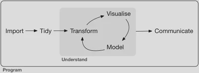
Rarely will your data arrive in exactly the form you require in order to analyze it appropriately. As part of the data science workflow you will need to transform your data in order to analyze it. Just as we established a syntax for generating graphics (the layered grammar of graphics), so too will we have a syntax for data transformation.

From the same author of ggplot2, I give you dplyr! This package contains useful functions for transforming and manipulating data frames, the bread-and-butter format for data in R. These functions can be thought of as verbs. The noun is the data, and the verb is acting on the noun. All of the dplyr verbs (and in fact all the verbs in the wider tidyverse) work similarly:

The first argument is a data frame
Subsequent arguments describe what to do with the data frame
The result is a new data frame

Key functions in `dplyr`

`function()`	Action performed
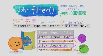
`filter()`	Subsets observations based on their values
`arrange()`	Changes the order of observations based on their values
`select()`	Selects a subset of columns from the data frame
`rename()`	Changes the name of columns in the data frame
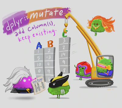
`mutate()`	Creates new columns (or variables)
`group_by()`	Changes the unit of analysis from the complete dataset to individual groups
`summarize()`	Collapses the data frame to a smaller number of rows which summarize the larger data

These are the basic verbs you will use to transform your data. By combining them together, you can perform powerful data manipulation tasks.

American vs. British English

Hadley Wickham is from New Zealand. As such he (and base R) favours British spellings:

The holy grail: "For consistency, aim to use British (rather than American) spelling." #rstats http://t.co/7qQSWIowcl. Colour is right!
— Hadley Wickham (@hadleywickham) November 27, 2013

While British spelling is perhaps the norm, this is America!

Fortunately many R functions can be written using American or British variants:

summarize() = summarise()
color() = colour()

Therefore in this class I will generally stick to American spelling.

Saving transformed data

dplyr never overwrites existing data. If you want a copy of the transformed data for later use in the program, you need to explicitly save it. You can do this by using the assignment operator <-:

filter(.data = diamonds, cut == "Ideal") # printed, but not saved

## # A tibble: 21,551 × 10
##    carat cut   color clarity depth table price     x     y     z
##    <dbl> <ord> <ord> <ord>   <dbl> <dbl> <int> <dbl> <dbl> <dbl>
##  1  0.23 Ideal E     SI2      61.5    55   326  3.95  3.98  2.43
##  2  0.23 Ideal J     VS1      62.8    56   340  3.93  3.9   2.46
##  3  0.31 Ideal J     SI2      62.2    54   344  4.35  4.37  2.71
##  4  0.3  Ideal I     SI2      62      54   348  4.31  4.34  2.68
##  5  0.33 Ideal I     SI2      61.8    55   403  4.49  4.51  2.78
##  6  0.33 Ideal I     SI2      61.2    56   403  4.49  4.5   2.75
##  7  0.33 Ideal J     SI1      61.1    56   403  4.49  4.55  2.76
##  8  0.23 Ideal G     VS1      61.9    54   404  3.93  3.95  2.44
##  9  0.32 Ideal I     SI1      60.9    55   404  4.45  4.48  2.72
## 10  0.3  Ideal I     SI2      61      59   405  4.3   4.33  2.63
## # … with 21,541 more rows

diamonds_ideal <- filter(.data = diamonds, cut == "Ideal") # saved, but not printed
(diamonds_ideal <- filter(.data = diamonds, cut == "Ideal")) # saved and printed

## # A tibble: 21,551 × 10
##    carat cut   color clarity depth table price     x     y     z
##    <dbl> <ord> <ord> <ord>   <dbl> <dbl> <int> <dbl> <dbl> <dbl>
##  1  0.23 Ideal E     SI2      61.5    55   326  3.95  3.98  2.43
##  2  0.23 Ideal J     VS1      62.8    56   340  3.93  3.9   2.46
##  3  0.31 Ideal J     SI2      62.2    54   344  4.35  4.37  2.71
##  4  0.3  Ideal I     SI2      62      54   348  4.31  4.34  2.68
##  5  0.33 Ideal I     SI2      61.8    55   403  4.49  4.51  2.78
##  6  0.33 Ideal I     SI2      61.2    56   403  4.49  4.5   2.75
##  7  0.33 Ideal J     SI1      61.1    56   403  4.49  4.55  2.76
##  8  0.23 Ideal G     VS1      61.9    54   404  3.93  3.95  2.44
##  9  0.32 Ideal I     SI1      60.9    55   404  4.45  4.48  2.72
## 10  0.3  Ideal I     SI2      61      59   405  4.3   4.33  2.63
## # … with 21,541 more rows

Do not use = to assign objects. Read this for more information on the difference between <- and =.

Using backticks to refer to column names

Normally within tidyverse functions you can refer to column names directly. For example,

count(x = diamonds, color)

## # A tibble: 7 × 2
##   color     n
##   <ord> <int>
## 1 D      6775
## 2 E      9797
## 3 F      9542
## 4 G     11292
## 5 H      8304
## 6 I      5422
## 7 J      2808

color is a column in diamonds so I can refer to it directly within count(). However this becomes a problem for any column name that is non-syntactic.¹ A syntactic name consists only of letters, digits, and . and _. Examples of non-syntactic column names include:

Social conservative
7-point ideology
_id

Any time you encounter a column that contains non-syntactic characters, you should refer to the column name using backticks ``.

count(x = diamonds, `color`)

## # A tibble: 7 × 2
##   color     n
##   <ord> <int>
## 1 D      6775
## 2 E      9797
## 3 F      9542
## 4 G     11292
## 5 H      8304
## 6 I      5422
## 7 J      2808

Do not use quotation marks ('' or "") to refer to the column name. This appears to work, but is not consistent and will fail when you do not expect it. Consider the same operation as above but using quotation marks instead of backticks.

count(x = diamonds, "color")

## # A tibble: 1 × 2
##   `"color"`     n
##   <chr>     <int>
## 1 color     53940

The word “color” has been duplicated 53940 times and tabulated using the count() function. Not what we intended. Always use the backticks for non-syntactic column names.

Missing values

NA represents an unknown value. Missing values are contagious, in that their properties will transfer to any operation performed on it.

NA > 5

## [1] NA

10 == NA

## [1] NA

NA + 10

## [1] NA

To determine if a value is missing, use the is.na() function.

When filtering, you must explicitly call for missing values to be returned.

df <- tibble(x = c(1, NA, 3))
df

## # A tibble: 3 × 1
##       x
##   <dbl>
## 1     1
## 2    NA
## 3     3

filter(df, x > 1)

## # A tibble: 1 × 1
##       x
##   <dbl>
## 1     3

filter(df, is.na(x) | x > 1)

## # A tibble: 2 × 1
##       x
##   <dbl>
## 1    NA
## 2     3

Or when calculating summary statistics, you need to explicitly ignore missing values.

df <- tibble(
  x = c(1, 2, 3, 5, NA)
)
df

## # A tibble: 5 × 1
##       x
##   <dbl>
## 1     1
## 2     2
## 3     3
## 4     5
## 5    NA

summarize(df, meanx = mean(x))

## # A tibble: 1 × 1
##   meanx
##   <dbl>
## 1    NA

summarize(df, meanx = mean(x, na.rm = TRUE))

## # A tibble: 1 × 1
##   meanx
##   <dbl>
## 1  2.75

Piping

As we discussed, frequently you need to perform a series of intermediate steps to transform data for analysis. If we write each step as a discrete command and store their contents as new objects, your code can become convoluted.

Drawing on this example from R for Data Science, let’s explore the relationship between the distance and average delay for each location. At this point, we would write it something like this:

by_dest <- group_by(.data = flights, dest)
delay <- summarise(
  .data = by_dest,
  count = n(),
  dist = mean(distance, na.rm = TRUE),
  delay = mean(arr_delay, na.rm = TRUE)
)
delay <- filter(.data = delay, count > 20, dest != "HNL")

ggplot(data = delay, mapping = aes(x = dist, y = delay)) +
  geom_point(aes(size = count), alpha = 1 / 3) +
  geom_smooth(se = FALSE)

## `geom_smooth()` using method = 'loess' and formula 'y ~ x'

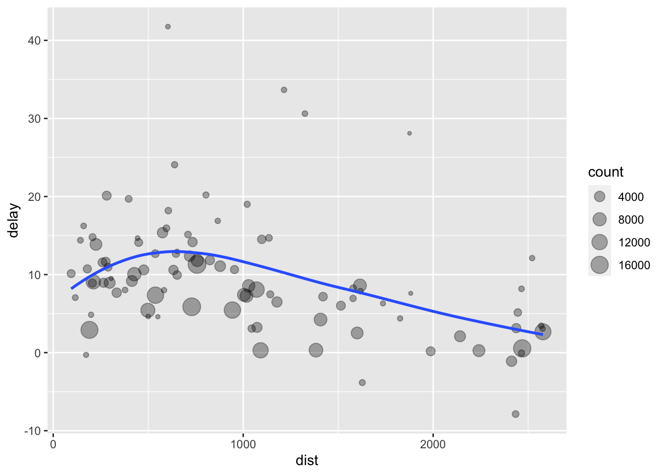
Decomposing the problem, there are three basic steps:

Group flights by destination.
Summarize to compute distance, average delay, and number of flights.
Filter to remove noisy points and the Honolulu airport, which is almost twice as far away as the next closest airport.

The code as written is inefficient because we have to name and store each intermediate data frame, even though we don’t care about them. It also provides more opportunities for typos and errors.

Because all dplyr verbs follow the same syntax (data first, then options for the function), we can use the pipe operator %>% to chain a series of functions together in one command:

delays <- flights %>%
  group_by(dest) %>%
  summarize(
    count = n(),
    dist = mean(distance, na.rm = TRUE),
    delay = mean(arr_delay, na.rm = TRUE)
  ) %>%
  filter(count > 20, dest != "HNL")

Now, we don’t have to name each intermediate step and store them as data frames. We only store a single data frame (delays) which contains the final version of the transformed data frame. We could read this code as use the flights data, then group by destination, then summarize for each destination the number of flights, the average disance, and the average delay, then subset only the destinations with at least 20 flights and exclude Honolulu.

Things to not do with piping

Remember that with pipes, we don’t have to save all of our intermediate steps. We only use one assignment, like this:

delays <- flights %>%
  group_by(dest) %>%
  summarize(
    count = n(),
    dist = mean(distance, na.rm = TRUE),
    delay = mean(arr_delay, na.rm = TRUE)
  ) %>%
  filter(count > 20, dest != "HNL")

Do not do this:

delays <- flights %>%
  by_dest() <- group_by(dest) %>%
  delay() <- summarize(
  count = n(),
  dist = mean(distance, na.rm = TRUE),
  delay = mean(arr_delay, na.rm = TRUE)
) %>%
  delay() <- filter(count > 20, dest != "HNL")

Error: bad assignment: 
     summarize(count = n(), dist = mean(distance, na.rm = TRUE), delay = mean(arr_delay, 
         na.rm = TRUE)) %>% delay <- filter(count > 20, dest != "HNL")

Or this:

delays <- flights %>%
  group_by(.data = flights, dest) %>%
  summarize(
    .data = flights,
    count = n(),
    dist = mean(distance, na.rm = TRUE),
    delay = mean(arr_delay, na.rm = TRUE)
  ) %>%
  filter(.data = flights, count > 20, dest != "HNL")

## Error in `filter()`:
## ! Problem while computing `..1 = .`.
## Caused by error in `summarize()`:
## ! Problem while computing `..1 = .`.
## Caused by error in `group_by()`:
## ! Must group by variables found in `.data`.
## ✖ Column `.` is not found.

If you use pipes, you don’t have to reference the data frame with each function - just the first time at the beginning of the pipe sequence.

Acknowledgments

Artwork by @allison_horst

Session Info

sessioninfo::session_info()

## ─ Session info ───────────────────────────────────────────────────────────────
##  setting  value
##  version  R version 4.2.1 (2022-06-23)
##  os       macOS Monterey 12.3
##  system   aarch64, darwin20
##  ui       X11
##  language (EN)
##  collate  en_US.UTF-8
##  ctype    en_US.UTF-8
##  tz       America/New_York
##  date     2022-10-05
##  pandoc   2.18 @ /Applications/RStudio.app/Contents/MacOS/quarto/bin/tools/ (via rmarkdown)
## 
## ─ Packages ───────────────────────────────────────────────────────────────────
##  package       * version    date (UTC) lib source
##  assertthat      0.2.1      2019-03-21 [2] CRAN (R 4.2.0)
##  backports       1.4.1      2021-12-13 [2] CRAN (R 4.2.0)
##  blogdown        1.10       2022-05-10 [2] CRAN (R 4.2.0)
##  bookdown        0.27       2022-06-14 [2] CRAN (R 4.2.0)
##  broom           1.0.0      2022-07-01 [2] CRAN (R 4.2.0)
##  bslib           0.4.0      2022-07-16 [2] CRAN (R 4.2.0)
##  cachem          1.0.6      2021-08-19 [2] CRAN (R 4.2.0)
##  cellranger      1.1.0      2016-07-27 [2] CRAN (R 4.2.0)
##  cli             3.4.0      2022-09-08 [1] CRAN (R 4.2.0)
##  codetools       0.2-18     2020-11-04 [2] CRAN (R 4.2.1)
##  colorspace      2.0-3      2022-02-21 [2] CRAN (R 4.2.0)
##  crayon          1.5.1      2022-03-26 [2] CRAN (R 4.2.0)
##  DBI             1.1.3      2022-06-18 [2] CRAN (R 4.2.0)
##  dbplyr          2.2.1      2022-06-27 [2] CRAN (R 4.2.0)
##  digest          0.6.29     2021-12-01 [2] CRAN (R 4.2.0)
##  dplyr         * 1.0.9      2022-04-28 [2] CRAN (R 4.2.0)
##  ellipsis        0.3.2      2021-04-29 [2] CRAN (R 4.2.0)
##  evaluate        0.16       2022-08-09 [1] CRAN (R 4.2.1)
##  fansi           1.0.3      2022-03-24 [2] CRAN (R 4.2.0)
##  farver          2.1.1      2022-07-06 [2] CRAN (R 4.2.0)
##  fastmap         1.1.0      2021-01-25 [2] CRAN (R 4.2.0)
##  forcats       * 0.5.1      2021-01-27 [2] CRAN (R 4.2.0)
##  fs              1.5.2      2021-12-08 [2] CRAN (R 4.2.0)
##  gargle          1.2.0      2021-07-02 [2] CRAN (R 4.2.0)
##  generics        0.1.3      2022-07-05 [2] CRAN (R 4.2.0)
##  ggplot2       * 3.3.6      2022-05-03 [2] CRAN (R 4.2.0)
##  glue            1.6.2      2022-02-24 [2] CRAN (R 4.2.0)
##  googledrive     2.0.0      2021-07-08 [2] CRAN (R 4.2.0)
##  googlesheets4   1.0.0      2021-07-21 [2] CRAN (R 4.2.0)
##  gtable          0.3.0      2019-03-25 [2] CRAN (R 4.2.0)
##  haven           2.5.0      2022-04-15 [2] CRAN (R 4.2.0)
##  here            1.0.1      2020-12-13 [2] CRAN (R 4.2.0)
##  highr           0.9        2021-04-16 [2] CRAN (R 4.2.0)
##  hms             1.1.1      2021-09-26 [2] CRAN (R 4.2.0)
##  htmltools       0.5.3      2022-07-18 [2] CRAN (R 4.2.0)
##  httr            1.4.3      2022-05-04 [2] CRAN (R 4.2.0)
##  jquerylib       0.1.4      2021-04-26 [2] CRAN (R 4.2.0)
##  jsonlite        1.8.0      2022-02-22 [2] CRAN (R 4.2.0)
##  knitr           1.40       2022-08-24 [1] CRAN (R 4.2.0)
##  labeling        0.4.2      2020-10-20 [2] CRAN (R 4.2.0)
##  lattice         0.20-45    2021-09-22 [2] CRAN (R 4.2.1)
##  lifecycle       1.0.2      2022-09-09 [1] CRAN (R 4.2.0)
##  lubridate       1.8.0      2021-10-07 [2] CRAN (R 4.2.0)
##  magrittr        2.0.3      2022-03-30 [2] CRAN (R 4.2.0)
##  Matrix          1.4-1      2022-03-23 [2] CRAN (R 4.2.1)
##  mgcv            1.8-40     2022-03-29 [2] CRAN (R 4.2.1)
##  modelr          0.1.8      2020-05-19 [2] CRAN (R 4.2.0)
##  munsell         0.5.0      2018-06-12 [2] CRAN (R 4.2.0)
##  nlme            3.1-158    2022-06-15 [2] CRAN (R 4.2.0)
##  nycflights13  * 1.0.2      2021-04-12 [2] CRAN (R 4.2.0)
##  pillar          1.8.1      2022-08-19 [1] CRAN (R 4.2.0)
##  pkgconfig       2.0.3      2019-09-22 [2] CRAN (R 4.2.0)
##  purrr         * 0.3.4      2020-04-17 [2] CRAN (R 4.2.0)
##  R6              2.5.1      2021-08-19 [2] CRAN (R 4.2.0)
##  readr         * 2.1.2      2022-01-30 [2] CRAN (R 4.2.0)
##  readxl          1.4.0      2022-03-28 [2] CRAN (R 4.2.0)
##  reprex          2.0.1.9000 2022-08-10 [1] Github (tidyverse/reprex@6d3ad07)
##  rlang           1.0.5      2022-08-31 [1] CRAN (R 4.2.0)
##  rmarkdown       2.14       2022-04-25 [2] CRAN (R 4.2.0)
##  rprojroot       2.0.3      2022-04-02 [2] CRAN (R 4.2.0)
##  rstudioapi      0.13       2020-11-12 [2] CRAN (R 4.2.0)
##  rvest           1.0.2      2021-10-16 [2] CRAN (R 4.2.0)
##  sass            0.4.2      2022-07-16 [2] CRAN (R 4.2.0)
##  scales          1.2.0      2022-04-13 [2] CRAN (R 4.2.0)
##  sessioninfo     1.2.2      2021-12-06 [2] CRAN (R 4.2.0)
##  stringi         1.7.8      2022-07-11 [2] CRAN (R 4.2.0)
##  stringr       * 1.4.0      2019-02-10 [2] CRAN (R 4.2.0)
##  tibble        * 3.1.8      2022-07-22 [2] CRAN (R 4.2.0)
##  tidyr         * 1.2.0      2022-02-01 [2] CRAN (R 4.2.0)
##  tidyselect      1.1.2      2022-02-21 [2] CRAN (R 4.2.0)
##  tidyverse     * 1.3.2      2022-07-18 [2] CRAN (R 4.2.0)
##  tzdb            0.3.0      2022-03-28 [2] CRAN (R 4.2.0)
##  utf8            1.2.2      2021-07-24 [2] CRAN (R 4.2.0)
##  vctrs           0.4.1      2022-04-13 [2] CRAN (R 4.2.0)
##  withr           2.5.0      2022-03-03 [2] CRAN (R 4.2.0)
##  xfun            0.31       2022-05-10 [1] CRAN (R 4.2.0)
##  xml2            1.3.3      2021-11-30 [2] CRAN (R 4.2.0)
##  yaml            2.3.5      2022-02-21 [2] CRAN (R 4.2.0)
## 
##  [1] /Users/soltoffbc/Library/R/arm64/4.2/library
##  [2] /Library/Frameworks/R.framework/Versions/4.2-arm64/Resources/library
## 
## ──────────────────────────────────────────────────────────────────────────────

See Advanced R for a more detailed discussion - but note that the book is called * Advanced R* for a reason. ↩︎

Last updated on Mar 1, 2019